the Creative Commons Attribution 4.0 License.
the Creative Commons Attribution 4.0 License.
 | 19 Aug 2024
Analysis of chi angle distributions in free amino acids via multiplet fitting of proton scalar couplings
Nabiha R. Syed
Nafisa B. Masud
Scalar couplings are a fundamental aspect of nuclear magnetic resonance (NMR) experiments and provide rich information about electron-mediated interactions between nuclei. 3J couplings are particularly useful for determining molecular structure through the Karplus relationship, a mathematical formula used for calculating 3J coupling constants from dihedral angles. In small molecules, scalar couplings are often determined through analysis of one-dimensional proton spectra. Larger proteins have typically required specialized multidimensional pulse programs designed to overcome spectral crowding and multiplet complexity. Here, we present a generalized framework for fitting scalar couplings with arbitrarily complex multiplet patterns using a weak-coupling model. The method is implemented in FitNMR and applicable to one-dimensional, two-dimensional, and three-dimensional NMR spectra. To gain insight into the proton–proton coupling patterns present in protein side chains, we analyze a set of free amino acid one-dimensional spectra. We show that the weak-coupling assumption is largely sufficient for fitting the majority of resonances, although there are notable exceptions. To enable structural interpretation of all couplings, we extend generalized and self-consistent Karplus equation parameterizations to all χ angles. An enhanced model of side-chain motion incorporating rotamer statistics from the Protein Data Bank (PDB) is developed. Even without stereospecific assignments of the beta hydrogens, we find that two couplings are sufficient to exclude a single-rotamer model for all amino acids except proline. While most free amino acids show rotameric populations consistent with crystal structure statistics, beta-branched valine and isoleucine deviate substantially.
- Article
(6360 KB) - Full-text XML
-
Supplement
(32806 KB) - BibTeX
- EndNote


The structure and dynamics of amino acid side chains are often critical for protein function. Side chains are not only an important part of the folded structure of proteins, but also key in facilitating molecular recognition, allosteric regulation, and catalysis. Nuclear magnetic resonance (NMR) is a particularly powerful technique for studying side chains as they move in solution at physiological temperatures. 3J scalar couplings give the most direct information about the local structure of side chains through the mathematical relationship between the dihedral angles of rotatable bonds and 3J, which was originally formulated by Karplus (1963). The numerous NMR experiments for measuring protein scalar couplings have been reviewed in detail by Vuister et al. (2002). Notably, it is possible to measure every scalar coupling involved in the side-chain χ1 angle, including 3J(HA–HB), 3J(C–HB), 3J(N–HB),3J(HA–CG), 3J(N–CG), and 3J(C–CG). (Protein Data Bank, PDB, atom names are used throughout this paper.)
Homonuclear proton–proton couplings, which are the focus of the present study, result in sometimes complex multiplet patterns in one-dimensional proton NMR spectra. Numerous pulse sequences have been developed to overcome this complexity and make proton–proton couplings easier to resolve and quantify in multidimensional spectra. The first was Exclusive Correlation Spectroscopy (E.COSY) (Griesinger et al., 1985, 1986, 1987), which generates cross-peak multiplets with reduced numbers of peaks and takes advantage of passive couplings to make line splitting by the active coupling visible for inspection and quantification. For 13C-labeled samples, this idea was extended using modified versions of the HCCH-COSY and HCCH-TOCSY experiments, where 1J(C–H) was used to resolve 3J(H–H) (Gemmecker and Fesik, 1991; Griesinger and Eggenberger, 1992; Emerson and Montelione, 1992). An HXYH experiment further improved experimental efficiency by simultaneously measuring both backbone and side-chain 3J couplings using 13C15N-labeled proteins (Tessari et al., 1995; Löhr et al., 1999). Another class of experiments, quantitative J correlation, uses the ratio between a diagonal and cross-peak to determine the value of the coupling constant, first demonstrated with the HNHA experiment, which measures the backbone 3J(H–HA) (Vuister and Bax, 1993). A HACACB-COSY adaptation of this technique enabled quantification of side-chain couplings (Grzesiek et al., 1995).
Another approach for obtaining scalar couplings uses numerical processing of a pair of matched experimental spectra, one having in-phase peaks with the same sign and the other having anti-phase peaks with opposite signs (Oschkinat and Freeman, 1984; Kessler et al., 1985; Titman and Keeler, 1990; Huber et al., 1993; Prasch et al., 1998). In these methods, a pair of trial anti-phase and in-phase peaks are convolved with a multiplet in the respective spectra. The coupling is determined by finding the separation between the trial peaks that results in maximum agreement between the two convolved spectra. However, peak overlap can be a problem with these types of methods because only a single multiplet is analyzed at a time.
Various approaches have been applied to directly fit peak multiplets that can handle peak overlap. SpinEvolution (Veshtort and Griffin, 2006), Quantum Mechanical Total Line Shape (QMTLS) fitting in PERCH (PERCH Solutions), ChemAdder (Tiainen et al., 2014), Guided Ideographic Spin System Model Optimization (GISSMO) (Dashti et al., 2017, 2018), ANATOLIA (Cheshkov et al., 2018), and Cosmic Truth (NMR Solutions) (Achanta et al., 2021) enable the fitting of a one-dimensional spectrum by iteratively optimizing parameters used to simulate the spectrum by a quantum mechanical description of the spin system(s) (Castellano and Bothner‐By, 1964; Heinzer, 1977; Cheshkov and Sinitsyn, 2020). Such calculations account for cases where the chemical shift difference between two nuclei approaches the value of their scalar coupling. This leads to strong coupling and the so-called “roofing effect”, where peaks in the multiplet closest to the other nucleus increase in intensity and those farthest decrease in intensity. While such calculations are usually computationally intensive, methods have been developed to very rapidly simulate one-dimensional spectra (Castillo et al., 2011). Global Spectral Deconvolution (GSD) in Mnova NMR (Mestrelab Research) enables fitting individual peaks in one-dimensional spectra and classification of peaks into multiplets (Bernstein et al., 2013). More recently, deep neural networks have been combined with line shape fitting to automatically quantify peaks in one-dimensional spectra (Li et al., 2023).
Several methods exist for fitting multidimensional spectra, including PINT (Ahlner et al., 2013; Niklasson et al., 2017) and INFOS (Smith, 2017), but those tools do not explicitly model scalar couplings. Amplitude-Constrained Multiplet Evaluation (ACME) was developed to fit proton–proton scalar couplings in COSY cross-peaks (Delaglio et al., 2001). Explicit modeling of scalar couplings in multidimensional spectra can also be done in Spinach (Hogben et al., 2011), which is a widely used software library optimized for simulations of large spin systems. However, like the commercially available NMRSim (Bruker) that can also simulate multidimensional spectra, the calculations can be time-consuming and are not typically used for direct spectral fitting.
Once accurate 3J couplings have been measured and quantified, they can be interpreted using the Karplus relationship, which relates 3J to a linear combination of cos θ and either cos 2θ or cos 2θ, where θ is the dihedral angle between the coupled nuclei. The three coefficients (a constant and two scaling factors for the cos functions) determine the Karplus parameterization. The coefficients for proteins have been most often determined using a large set of scalar coupling measurements for which coordinates from X-ray crystallography are also available. A structure-free approach to parameterizing scalar couplings was developed by Schmidt et al. (1999). It depends on the measurement of many different scalar couplings, each with a different relationship to the overall dihedral angle. By having many scalar couplings, both the dihedral angles of the chemical bonds and the associated Karplus parameters can be determined in a self-consistent manner. This approach was originally applied to scalar couplings in the protein backbone (Schmidt et al., 1999) and then expanded to side chains (Pérez et al., 2001). A model known as the generalized Karplus equation was parameterized 2 decades earlier primarily using data from small molecules with six-membered rings (Haasnoot et al., 1979, 1980, 1981a, b). This approach used a formula incorporating differences in the electronegativity between hydrogen and the substituted heavy atoms, the orientation of the substituent relative to the hydrogen, and the electronegativities of secondary substituents.
One of the first studies into the conformational preferences of amino acids using scalar couplings examined the effect of N- and C-terminal charge states on the rotamer equilibrium (Pachler, 1963). For individual amino acids, the ContinUous ProbabIlity Distribution (CUPID) method was developed that also incorporated information from nuclear Overhauser effect experiments (Dzakula et al., 1992). That and numerous other methods for analyzing scalar coupling data to determine dihedral angles and distributions have been reviewed (Kraszni et al., 2004). Scalar couplings are also used to determine conformational ensembles of proteins using the standard and generalized Karplus equations (Steiner et al., 2012). In the context of full proteins, molecular-dynamics-enhanced sampling techniques have been shown to improve convergence and fit to experimental data (Smith et al., 2021). Beyond scalar couplings, residual dipolar couplings have also been used to analyze side-chain conformations in folded proteins (Mittermaier and Kay, 2001; Li et al., 2015).
The 3J(H–HA) scalar coupling is dependent on the phi backbone dihedral angle and takes distinct values depending on whether the residue is part of an alpha helix or beta sheet. In most heteronuclear NMR spectra, the power output required for decoupling 13C and/or 15N in isotopically labeled proteins limits the direct-dimension acquisition time, leading to signal truncation that hinders the resolution of the 3J(H-HA) line splitting. Increasing molecular size also broadens the line widths, further exacerbating the resolution. However, we recently showed that through very precise modeling of signal truncation and apodization, 3J(H-HA) could be quantified in the ordinary 1H−15N two-dimensional spectra using nonlinear least-squares fitting in FitNMR (Dudley et al., 2020). A byproduct of this fitting is that the 1H transverse relaxation rate, , can also be quantified, which can provide valuable information about protein structure and dynamics (Dudley et al., 2024).
Towards the ultimate goal of being able to similarly quantify side-chain 1H scalar couplings and values directly from multidimensional spectra of folded proteins as well as extract accurate volumes for clearly overlapping peaks, we present an analysis of the proton–proton couplings in 1H spectra of individual amino acids. We describe how FitNMR was enhanced to directly model complex multiplet patterns in multidimensional spectra using a simple tabular input/output format. The strengths and weaknesses of using a model that assumes purely weak-coupling interactions are illustrated. To obtain Karplus parameters, we extend a self-consistent parameterization of 3J(HA–HB) couplings to include 3J(HB–HG), 3J(HG–HD), and 3J(HD–HE). Finally, we apply an enhanced model of side-chain motion incorporating prior rotameric information to determine differences in the conformational preferences between the side chains of free amino acids and those found in crystal structures.
2.1 Fitting couplings in multidimensional spectra
FitNMR (Dudley et al., 2020) was originally designed such that each peak in a multiplet would be a distinct entity. To allow for scalar couplings, the chemical shifts in a given peak could be made a linear combination of auxiliary chemical shift parameters, whose coefficients were chosen such that a scalar coupling in hertz could be mapped onto the parts per million scale. While this functioned well for fitting simple doublets found in protein 1H−15N two-dimensional spectra, it did not scale well to other applications, especially complicated spectra with heterogeneous coupling patterns.
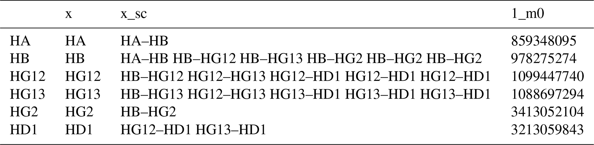
To address this, we developed a new way of defining NMR spectral features, for which we use the term resonances. They are defined in a comma separated values (CSV) resonances text file, with an example for isoleucine shown in Table 1. The first column gives the name of the resonance, which can be arbitrarily defined. FitNMR supports up to four spectral dimensions, referred to using the names x, y, z, and a, following nomenclature used by NMRPipe (Delaglio et al., 1995). The particular nucleus associated with each dimension is given in the column with the same name as the dimension. Scalar couplings active in each dimension are given in a corresponding column whose name has the _sc suffix. They are space-delimited and can also be arbitrarily named, although no nucleus and scalar coupling may share the same name. A scalar coupling can appear several times to produce canonical multiplets like triplets and quartets. For instance, in isoleucine, the HB resonance definition produces a doublet of doublets of doublets of quartets, with couplings to HA, HG12, and HG13 each producing a doublet and couplings to the HG2 methyl group producing a quartet. Additional columns give the volumes associated with individual spectra, referred to by FitNMR as m0 (initial magnetization).
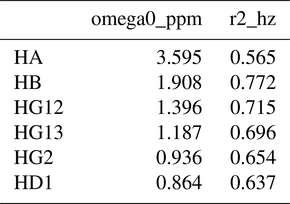

Each nucleus referred to in the resonances table is defined in the nuclei table, with an example for isoleucine shown in Table 2. The first column gives the nucleus name. The second, omega0_ppm, column gives the chemical shift offset, Ω0, in parts per million. The third r2_hz column gives the transverse relaxation rate (including an inhomogeneous contribution), , in hertz. The coupling table (Table 3) just has a single hz data column, with the value of the scalar coupling in hertz. Because they are associated with saturated carbons, all 2J couplings are assumed to be negative. However, in the present work, the sign has no impact because all couplings are in phase. CSV files for all fitted parameters are available in the data/fit1d_fitnmr_output.tar.gz file within the Supplement ZIP archive.
2.2 Fitting amino acid one-dimensional spectra
Starting parameters for fitting amino acid one-dimensional NMR spectra were adapted from the Guided Ideographic Spin System Model Optimization (GISSMO) database (Dashti et al., 2017, 2018), with couplings added or removed as appropriate. Chemical shifts were manually altered to account for differences in referencing and effects of strong coupling, which FitNMR does not currently model. Standard PDB atom names were used. When two nonmethyl protons were modeled with a single chemical shift, their respective numbers were separated by a slash. For methyl protons, the last number identifying each proton was dropped from the name. Geminal proton names were assigned to follow the ordering observed in the Biological Magnetic Resonance Data Bank (BMRB) statistics (https://bmrb.io/histogram/, last access: 1 April 2024) and do not reflect a stereospecific analysis of the fitted 3J coupling values.
Fitting was done with the refit_peaks.R script from FitNMR 0.7. The spectra were fit in a region of ±0.02 ppm from the starting peaks in each multiplet. The chemical shift was allowed to move up to 3.5 times the starting during fitting. was constrained to being 0.1 to 2 Hz, and the scalar couplings were constrained to be −20 to 20 Hz.
2.3 Karplus parameters for side-chain χ angles
When spanning a rotatable bond, 3J scalar couplings provide information about the dihedral angle (θ) between the two coupled atoms through the well-known Karplus relationship (Karplus, 1963):
An alternative formulation of the Karplus relationship dependent on cos θ and cos 2θ terms is often used. Here, we apply two enhanced forms of the Karplus equation, one that is known as the generalized Karplus equation (Haasnoot et al., 1980) and another which we will refer to as the self-consistent Karplus equation (Pérez et al., 2001). In this work, both are applied to dihedral angles in protein side chains. The generalized Karplus equation (Haasnoot et al., 1980) is
The terms give the electronegativity difference between the four other substituent groups (S1 to S4) bonded to the central C1−C2 atom pair. They are calculated using the difference in Huggins electronegativity (Huggins, 1953) between hydrogen and the α atom (bonded to C1 or C2) and β atoms (bonded to the α atom) in each substituent group:
Here, we follow the geometric standard described by Haasnoot et al. (1980), where S1 and S2 are bonded to C1, with S1 directly clockwise from H1 on a Newman projection, with C1 in front of C2, and S2 directly counterclockwise from H1. S3 and S4 are directly clockwise and counterclockwise, respectively, from H2 on a Newman projection, with C2 in front of C1. ξi gives the sign of rotation and is +1 for and −1 for .
Parameters P1 to P7 were derived from fits to couplings in primarily six-membered ring structures with restricted geometries (Haasnoot et al., 1980). Parameter set B (P1=13.7, , P3=0, P4=0.56, , P6=16.9°, and P7=0.14) was derived from couplings with two to four substituents. Parameter set D (P1=13.22, , P3=0, P4=0.87, , P6=19.9°, and P7=0) was derived from couplings with three substituents. Parameter set E (P1=13.24, , P3=0, P4=0.53, , P6=15.5°, and P7=0.19) was derived from couplings with four substituents. Here, we follow recommendations by Haasnoot et al. (1980) using parameter sets B, D, and E for couplings with two, three, and four substituents, respectively.
For this work, we determined the complete set of parameters ( to ) necessary for a generalized Karplus analysis of proton–proton couplings associated with χ1–4 by analyzing representative amino acid structures taken from the PDB Chemical Component Directory (CCD) (Westbrook et al., 2015). An example representative structure for isoleucine is shown in Fig. 1a, and the parameters determined for all amino acids are given in Table A2 in Appendix A.
The self-consistent Karplus equation (Schmidt et al., 1999) perturbs the average scalar coupling given by the C0 coefficient in Eq. (1) using a set of increments (ΔC0,i) weighted by the number (Ni) of proton/heavy-atom α substitutions made around the bond for a particular element type i:
This formulation makes it possible to extrapolate the parameterization to chemical substructures outside the training set. For side-chain proton–proton 3J couplings, the following previously determined (Pérez et al., 2001) coefficients and coefficient increments were used: C0=7.24, , C2=3.61, , , and Hz. The offset for nitrogen atoms was previously defined as Hz because NN=1 for all side-chain χ1 angles, making it impossible to separate the contribution of a nitrogen substitution from the fundamental Karplus coefficient, C0. For the χ1 dihedral angle, the heavy-atom substitution counts were previously published (Pérez et al., 2001). Here, we determined the number of α substituents for proton–proton couplings associated with χ1–4, which are given in given in Table A3.
In Eqs. (1), (2), and (4), the θ angle refers to the dihedral angle between the two coupled protons, which is often offset from the canonical side-chain χ angle (χ) by a given value, Δχ:
In this paper, whenever the χ symbol has a superscript (like g, α, or β), it refers to electronegativity. All other instances of χ refer to side-chain dihedral angles. Using the CCD representative amino acid structures, we determined Δχ offsets (rounded to −120, 0, and 120°) for χ angles 1–4, which are given in given in Tables A2 and A3.
A comparison of the generalized and self-consistent Karplus equations is shown in Fig. A1 in Appendix A. Over the nine sets of unique self-consistent parameters, the range of coupling values sampled by the generalized parameters is 2.7 Hz greater on average than the self-consistent parameters. Although the generalized Karplus equation was parameterized on bonds geometrically restricted by rings, the self-consistent equation was parameterized using data from a protein in solution. While efforts were made to account for the effects of protein motional averaging in the self-consistent parameterization (see below), it could be that the degree of protein motion was underestimated, resulting in less extreme Karplus curves in order to reproduce the measured scalar couplings. The generalized parameters also produce slightly higher couplings overall, with an average coupling value 0.6 Hz greater than the self-consistent parameters. Finally, averaging over the nine sets, there is a 1.5 Hz root mean square deviation between the couplings produced by the two equations.
2.4 χ angle distribution analysis
During self-consistent parameterization of the side-chain Karplus parameters (Pérez et al., 2001), two different models of motion were previously used. Model M1 involved normally distributed fluctuation about a mean χ1 angle with standard deviation . Model M2 assumed jumps between 60, 180, and 300° and varied the respective populations. Each model had two free parameters, and M1 was used for determining the final published parameters.
Here, we also apply a third model (which we call M3) involving jumps between three rotameric bins, whose χ angle distributions were taken from the 2010 Dunbrack rotamer library (Shapovalov and Dunbrack, 2011). The M3 model used 610 177 different side-chain conformations from their dataset. For each side-chain conformation, the theoretical coupling value was calculated using Eq. (4) and the data from Table A3. Depending on the application, these theoretical couplings were averaged over all rotamers (as done for Fig. 3) or the three different rotameric bins associated with χ1 (as done for Fig. 5).
3.1 Fitting amino acid one-dimensional spectra
To gain an insight into coupling patterns between carbon-bound protons in amino acid side chains, we performed fits of spectra taken from the Biological Magnetic Resonance Data Bank (BMRB) (Hoch et al., 2023) (Table A1). The samples contained individual amino acids dissolved in D2O, nearly eliminating peaks from solvent and exchangeable protons. A representative fit for isoleucine is shown in Fig. 1. The resonances are defined as shown in Table 1 and parameters derived from the fit are shown in Tables 1–3. The HA, HG2, and HD1 resonances are each affected by only one or two 3J couplings, making their relatively simple multiplet patterns easy to resolve. The HG12 and HG13 resonances add a mutual 2J coupling and a 3J coupling to the HB atom. The HG12/HG13 chemical shift difference of 104.7 Hz (relative to the −13.5 Hz 2J coupling) is sufficient to minimize roofing effects from strong coupling in the experimental data (black), which shows minimal deviation from the modeled contribution of each resonance (gray and yellow, respectively). Despite a very complicated multiplet pattern for the HB atom (a doublet of doublets of doublets of quartets; blue), the resonance is very well fit by the model due to the couplings being shared with resonances having much less complexity.
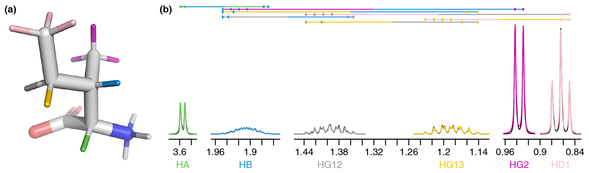
Figure 1(a) Representative structure of isoleucine taken from the CCD with the termini made zwitterionic in PyMOL. Protons are grouped by color, with each color having a distinct chemical shift modeled by a single resonance in the fit. The hydrogens (white) are deuterated due to exchange with D2O. (b) Fit of 500 MHz 1H NMR spectrum of isoleucine in D2O as described by Tables 1–3. The experimental spectrum is shown in black, and the modeled signal corresponding to each resonance is shown with the same color as in (a). Each scalar coupling is represented by a horizontal line above the spectrum, with the colors matched to the group being coupled to. The outermost multiplet produced by each coupling is represented by vertical dashes. The x axis gives the 1H chemical shift in parts per million using sparse representation. This panel was produced with the plot_sparse_1d FitNMR function.
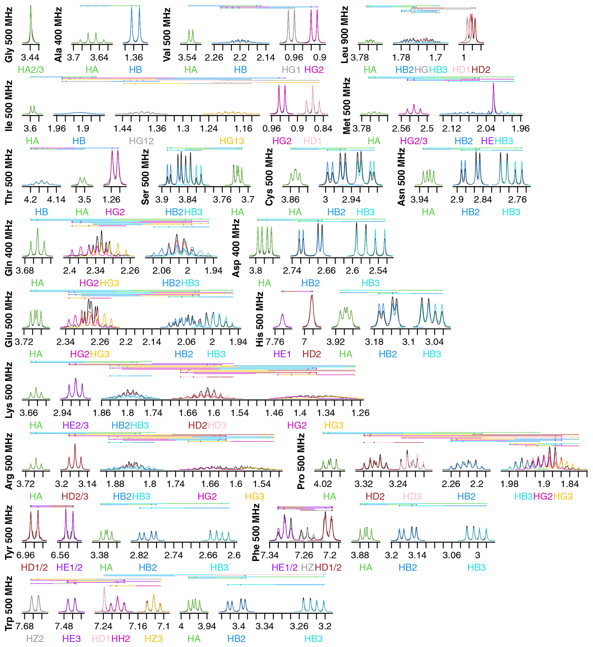
Figure 2Fits of 1H NMR spectra of all 20 canonical amino acids in D2O. Spectra are plotted as described in Fig. 1. The total modeled sum of all resonance contributions is shown in red, which is usually obscured by the individual contributions.
Fits for all 20 amino acids are shown in Fig. 2. Similar to isoleucine, the relatively simple spectra for glycine, alanine, valine, and threonine are all fit quite well and do not show significant strong coupling effects. The same is true of tryptophan, which has eight distinct resonances but only very slight strong coupling between HB2 and HB3.
Strong coupling is more pronounced in the beta protons of serine, cysteine, asparagine, and aspartate. These four side chains have the same three protons in the spectra, with HB2 and HB3 showing significant roofing effects. However, the multiplet patterns are easily resolved, and the weak-coupling model used by FitNMR finds an intermediate intensity between the two doublets. Despite not modeling the roofing effect, the line widths do not appear to be distorted by the intensity mismatch. Histidine is largely similar with the addition of HD2 and HE1 nuclei in the imidazole ring that are only coupled to one another via a 1.7 Hz 4J coupling.
Glutamine and glutamate add HG2 and HG3 nuclei, each with similar but distinct chemical shifts, leading to large strong coupling effects. This results in outer multiplet peaks nearly disappearing. In proline, the HG2 and HG3 nuclei also have very similar chemical shifts and are quite strongly coupled. For methionine, the HG2 and HG3 nuclei appear to have indistinguishable chemical shifts and very similar scalar couplings, producing two overlapping, near-canonical triplets.
Leucine, with one HG atom, has two terminal methyl groups, each represented by a single resonance (HD1 or HD2). These make the multiplet pattern for HG quite complex. Due to the very similar 3J(HG–HD1) and 3J(HG–HD2) coupling constants (6.6 and 6.5 Hz, respectively), it is essentially a doublet of doublets of septets. Together with significant overlap between HB2, HB3, and HG (forming a strong coupling network between the three nuclei), this makes fitting the spectrum in this region very difficult. However, it is made somewhat easier because couplings involving the more isolated HA, HD1, and HD2 can be more easily resolved.
Tyrosine and phenylalanine also have somewhat complicated coupling networks in their aromatic rings, with four and five strongly coupled nuclei, respectively. They should each theoretically have both 3J(HD1–HE1 or HD2–HE2) and 5J(HD1–HE2 or HD2–HE1) couplings. In a purely weak-coupling model neglecting couplings between equivalent nuclei, that would create a doublet of doublets for HD1/2 and HE1/2 in tyrosine. However, the experimental spectrum (black) resembles a doublet of triplets. The outer peaks in each triplet have much lower intensities than a classic 1 : 2 : 1 triplet and exhibit roofing. Accurate modeling of this requires separate quantum mechanical treatment of the spin states of HD1, HD2, HE1, and HE2. During fitting, 5J(HD–HE) drops to less than 0.0001 Hz, represented by the topmost vertical line. The phenylalanine fit does obtain reasonable values of 1.2 and 0.7 Hz for 5J(HD–HE) and 4J(HD–HZ), respectively. However, triplet behavior is still observed in the experimental spectrum, particularly for HE1/2, and remains unexplained by the weak-coupling model.
Lysine, arginine, and proline are all capable of having distinct proton chemicals shifts at the beta, gamma, and delta positions. Distinct chemical shifts are observed for all such protons except for the HD2 and HD3 atoms in arginine. They show identical chemical shifts and produce a near-perfect triplet, suggesting that the scalar couplings they make with HG2 and HG3 rotationally average out to near-identical values. The values of those scalar couplings and rotational averaging will be discussed in more detail below. While nearly all resonances in proline are modeled well, lysine and arginine are more difficult, especially for the HG2 and HG3 atoms, each of which are coupled to five nuclei.
Our data show that the large majority of protons in amino acid side chains can be modeled well using the FitNMR weak-coupling approximation. However, peak overlap is an issue for several nuclei, suggesting two-dimensional proton spectra like a nuclear Overhauser effect spectroscopy (NOESY) or double-quantum-filtered COSY (DQF-COSY) may be required for adequate resolution. In addition, FitNMR and similar methods would benefit from the incorporation of quantum mechanical calculations to enable accounting for strong coupling in the spectra.
3.2 χ-angle-dependent side-chain scalar couplings
Karplus parameters are required to derive structural information from scalar couplings. For 3J couplings between adjacent CH2 groups, the four proton–proton couplings completely sample all three values of Δχ (see χ2–4 parameters in Tables A2 and A3), providing detailed structural information. To use the generalized Karplus equation, we calculated the required electronegativity differences and positions of all substituent groups (Table A2). For the self-consistent Karplus equation, we extrapolated parameters derived from scalar couplings associated with χ1 (Pérez et al., 2001) to χ2–4 (Table A3). We did not attempt a reparameterization of C0 and ΔC0,N (see Methods, Sect. 2.3) to account for the absence of a nitrogen substitution at χ2 (in leucine, isoleucine, methionine, glutamine, glutamate, lysine, arginine, and proline) or χ3 (in lysine).
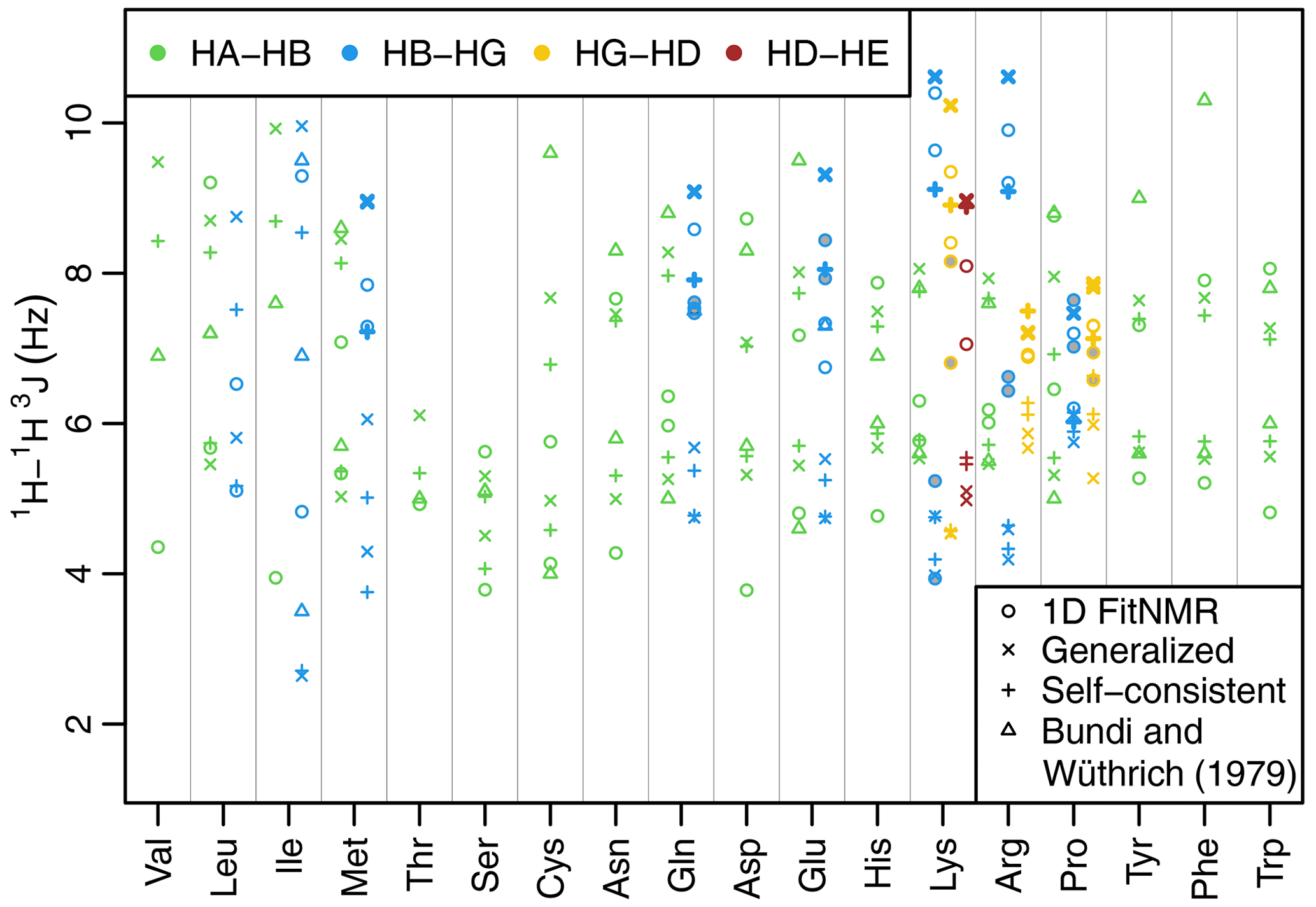
Figure 3Side-chain 1H−1H 3J scalar couplings that depend on χ angles through the Karplus relationship. Couplings from fits of the one-dimensional NMR spectra are shown with circles. Theoretical couplings calculated from the dataset used to create the 2010 Dunbrack rotamer library are shown with an × (using generalized Karplus equation) or a plus sign (using self-consistent equation). Experimental couplings from GGXA tetrapeptides (Bundi and Wüthrich, 1979) are shown with triangles. HA–HB couplings are shown in green, HB–HG couplings are shown in blue, HG–HD couplings are shown in yellow, and HD–HE couplings are shown in auburn. The dihedral angles governing 3J(HB2–HG2) and 3J(HB3–HG3) have the same Δχ (see Methods and Tables A2 and A3) and therefore have the same theoretical value shown with a thick × or plus sign. The same is true for the corresponding HG–HD and HD–HE couplings. Experimental couplings between speculatively assigned atoms 2–2 and 3–3 of adjacent methylene groups are shaded gray. Depending on the actual assignments, either the shaded or the unshaded pair of experimental couplings should correspond to the theoretical couplings indicated with the thick symbols.
The fit-derived 3J couplings dependent on a side-chain χ angle are shown as circles in Fig. 3. There are eight amino acids with χ2-related couplings (blue), three amino acids with χ3-related couplings (yellow), and one with χ4-related couplings (auburn). For χ angles with CH2 groups on both sides of the associated rotatable bond, there are two couplings that in principle should take the same value due to having the same Δχ offset (see Methods, Tables A2 and A3, and Fig. A1h and i for possible exceptions). These scalar couplings were obtained without any constraint on their similarity in the software nor human knowledge of the expected equivalence during manual optimization of the input parameters. Despite that and the lack of stereospecific assignments, such equivalent couplings were within about 1 Hz of each other in all but one case (lysine HG–HD), supporting the relative accuracy of our approach despite the limitations.
As an initial point of comparison, we used the 2010 Dunbrack rotamer library dataset to calculate theoretical scalar couplings assuming the same χ angle distributions observed in crystal structures. In Fig. 3, these are shown using either an × (calculated using generalized Eq. 2) or a plus sign (calculated with self-consistent Eq. 4). For the calculated rotamer library couplings, thick symbols represent the two scalar couplings with equivalent Δχ offsets. If our speculative stereospecific assignments for both methylene protons are either both correct or both incorrect, this pair of geometrically equivalent experimental coupling values are shown as shaded circles. Alternatively, if only one of the methylene assignments is incorrect, then the unshaded circles should be equivalent. For these geometrically equivalent couplings, the experimental and rotamer library couplings are generally within about 1.5 Hz of each other. As noted above, there are possible exceptions to the coupling equivalence that happen due to geometric relationships between electron-withdrawing groups and the coupled protons (Haasnoot et al., 1980), which is accounted for by the generalized Karplus equation. However, the only angle where this is observable in our simulated couplings is at proline χ3 (see the two distinct thick yellow × symbols for proline in Fig. 3 and phase-shifted solid lines in Fig. A1i).
Beta-branched amino acids have just a single coupling associated with χ1, allowing unambiguous comparison. Of these, the experimental and rotamer library couplings are very similar for threonine. However, the couplings for valine and isoleucine are quite different, suggesting that some combination of the charged termini, absence of neighboring amino acid residues, or solvent exposure alters the free energy of these hydrophobic residues when free in solution. For valine and isoleucine, GGXA tetrapeptide couplings (Bundi and Wüthrich, 1979) are closer to the rotamer-library-derived couplings than the free amino acid couplings. For other residues, notably cysteine, glutamate, tyrosine, and phenylalanine, one of the tetrapeptide couplings is much higher than any of the free amino acid or rotamer couplings.
Many of the experimentally measured scalar couplings with ambiguous assignments have rotamer library values somewhat nearby, providing less support for (but not necessarily excluding) differences in the energetic preferences. One possible systematic divergence between the experimental and rotamer-derived couplings was in the absolute difference between the two HA–HB couplings, , which is especially pronounced for aspartate. However, with the experimental Δ3J(HA–HB) value being greater than the rotamer library value (calculated using self-consistent Eq. 4) for 10 out of 15 residues, the difference was not statistically significant (p=0.20). Likewise, using generalized Karplus Eq. (2) to calculate rotamer library values, only 8 out of 15 residues showed a larger experimental coupling range (p=0.80).
3.3 Analysis of χ1 angle distributions
To more quantitatively model distributions of the χ1 angle, for which the most reliable Karplus parameters were available, we used several different models of motion. The first, M1, models χ angle fluctuations as being normally distributed with standard deviations ranging from 0–50°. During development of the self-consistent Karplus parameters, both the Karplus parameters and the M1 model parameters (χ1 and ) describing each experimentally measured residue were jointly optimized to be self-consistent with one another (Pérez et al., 2001).
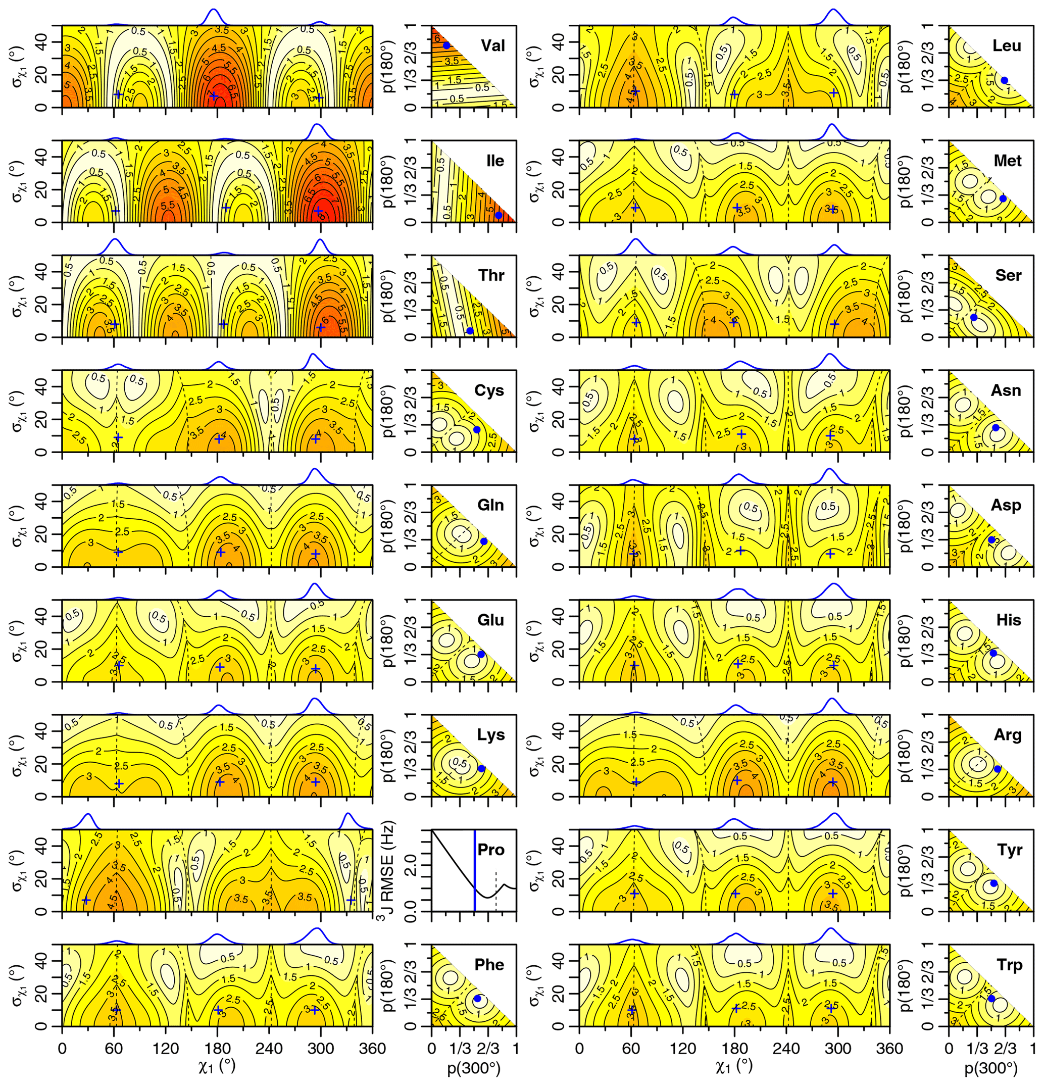
Figure 4Generalized Eq. (2) 3J(HA–HB) root mean squared error (RMSE) in hertz for M1 (left) and M3 (right) models of motion. Dashed lines separate regions with swapped assignments. Dunbrack rotamer library distributions are shown on top of the M1 plots, with the M1 model having the closest match to each shown with a blue plus sign. Rotamer library populations are shown as a blue point or solid vertical line in the M3 plots.
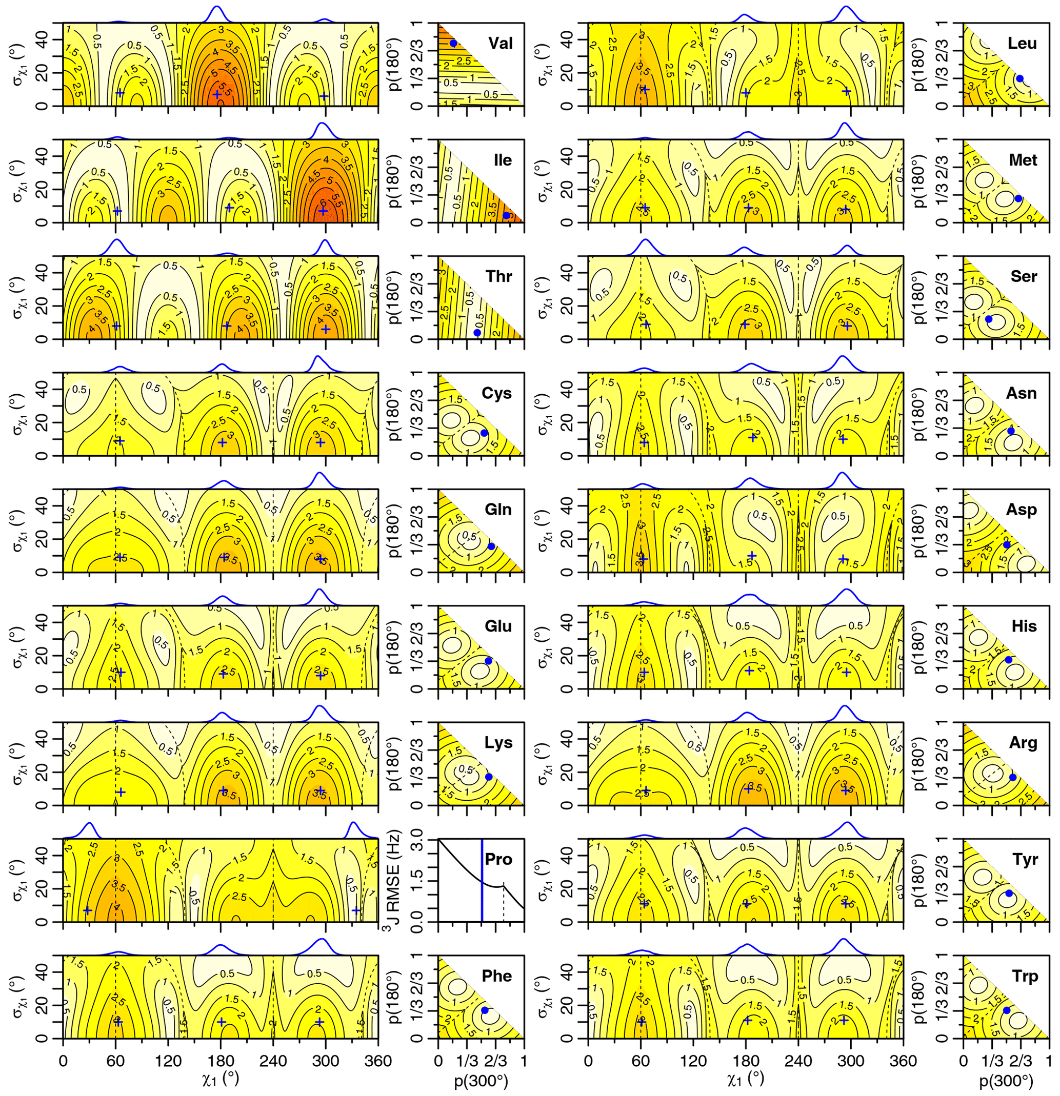
Figure 5Self-consistent Eq. (4) 3J(HA-HB) root mean squared error (RMSE) in hertz for M1 (left) and M3 (right) models of motion. Dashed lines separate regions with swapped assignments. Dunbrack rotamer library distributions are shown on top of the M1 plots, with the M1 model having the closest match to each shown with a blue plus sign. Rotamer library populations are shown as a blue point or solid vertical line in the M3 plots.
For the full range of χ1 and values, we calculated the root mean squared error (RMSE) between the back-calculated and experimentally measured scalar couplings. Those are shown as rectangular contour plots in Fig. 4 (generalized Eq. 2) and Fig. 5 (self-consistent Eq. 4). For the evaluation of the different models, we made no assumption about the stereospecific assignments of the HB2 and HB3 atoms. The RMSE values were calculated for both possible assignments, and the minimum RMSE for a given set of model parameters is shown. Boundaries between regions with different assignments are drawn as dashed lines. For the beta-branched amino acids (valine, isoleucine, and threonine), there is no such ambiguity, but the single scalar coupling provides less information.
The χ1 distributions used by the Dunbrack rotamer library are shown in blue on top of each contour plot. For reference, we determined the M1 model parameters that produced the closest distribution (in terms of the Bhattacharyya distance) to each rotameric bin distribution. Those parameters are shown with blue plus signs. For amino acids excluding proline, the mean angles matching the rotamer library distributions (ranging from 61–66, 176–190, and 291–300°) were close to the canonical values. Due to the need for ring closure, the proline χ1 angle distributions are skewed towards 0 or 360° and report primarily on ring pucker. The standard deviations of the rotamer library distributions ranged 6–11°, with aromatic side chains having the most variation (°).
While was varied, 0–50°, both here and in the self-consistent Karplus parameterization, values much greater than those observed in the PDB are not physically realistic. Furthermore, mean angles too far from those observed in the PDB are also not likely. The applicability of the unimodal M1 model to the experimental data can be judged based on how nearby a region with low RMSE is to the blue plus sign. For nearly all of the amino acids, the measured 3J(HA–HB) couplings are sufficient to exclude the M1 model, suggesting that they instead populate multiple rotamer bins, as would be expected for an free amino acid in solution. Proline does show a set of M1 parameters with low self-consistent RMSE values very close to a rotamer library distribution. Isoleucine is the only other amino acid where the single-rotamer model could be considered reasonable (with a plus symbol RMSE < 1 Hz), likely due to the reduced information content of the single scalar coupling.
An alternate M2 model was previously tested that back-calculated the scalar couplings using a population-weighted mean of the theoretical scalar couplings at 60, 180, and 300°, which also makes it a two-parameter model (Pérez et al., 2001). However, as the Dunbrack rotamer library indicates, side chains generally sample a range of values within a rotamer well. In addition, there is an amino-acid-specific bias away from the canonical angles, which can be subtle for many amino acids but quite large for proline. To account for this prior information, we propose another two-parameter model, referred to here as M3, that uses average scalar couplings calculated directly from the rotameric bins in the Dunbrack 2010 rotamer library dataset.
The RMSE values for the M3 model are shown as square contour plots in Figs. 4 and 5, with the populations from the rotamer library shown as a blue point. Because only two valid rotamers exist for proline, the RMSE is plotted as a line against the population of the 300° (gauche minus) rotamer bin, with the rotamer library population shown as a vertical blue line.
For the M1 model, which allows χ angles with unrealistically high potential energies, it is possible to judge model applicability by comparing it with rotamer library distributions (i.e., blue plus signs). However, because the M3 model stays within observable χ angles by definition, there is not necessarily a means to assess model validity with a priori information. However, the vast majority of free amino acids do have scalar couplings reasonably consistent (RMSE < 1.5 Hz) with the rotamer library populations, which is not necessarily expected given the presence of the and COO− groups, lack of neighboring amino acids, and high solvent exposure.
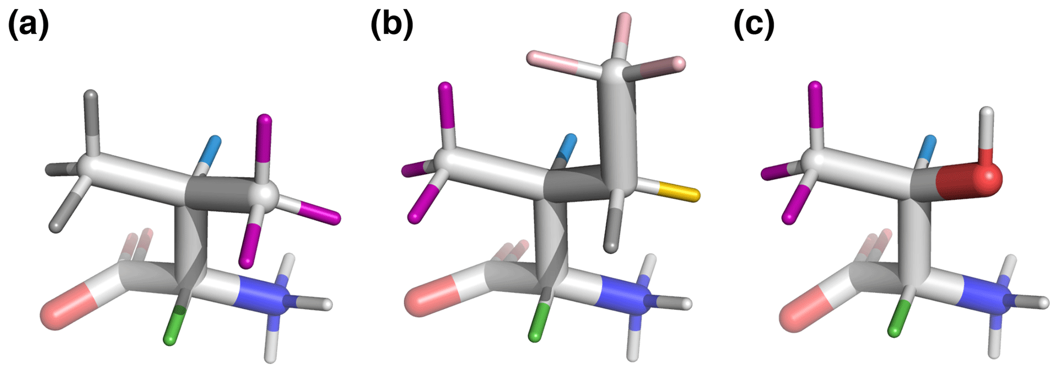
Figure 6Beta-branched amino acids, with hydrogen colors matching those used in Figs. 1 and 2. 3J(HA–HB) is most sensitive to the population of the shown rotamers because HA (green) is trans to HB (blue), giving the maximum theoretical scalar coupling. (a) Valine, χ1=180°, rotamer. (b) Isoleucine, χ1=300°, rotamer. (c) Threonine, χ1=300°, rotamer. Hydroxyl hydrogen (white) was also deuterated in the sample.
By contrast, beta-branched valine and isoleucine have 3J(HA–HB) values (4.4 and 3.9 Hz, respectively) that are quite inconsistent with the rotamer populations observed in the PDB. The χ1=180° rotamer of valine and χ1=300° rotamer of isoleucine, both highly populated in the PDB, have very similar three-dimensional structures due to differences in the way χ1 atoms are defined (Fig. 6a, b). These rotamers are likely very prevalent in folded proteins because they avoid more strained conformations where either gamma carbon has two gauche interactions with the backbone. Interestingly, the threonine χ1=300° rotamer that has a similar heavy-atom arrangement (Fig. 6c) appears to have a 20 %–45 % population in solution according to the M3 model (Figs. 4 and 5). The differences in preferences for these rotamers in the free amino acids could arise due to the more hydrophobic side chains of valine and isoleucine imposing a greater desolvation penalty on the group than threonine does. The greater similarity of the GGXA tetrapeptide couplings to those from the rotamer library supports this mechanism (Fig. 3).
Proline is another amino acid whose PDB populations show varying levels of consistency with those observed for the free amino acid. Crystal structures show nearly equal populations of the Cγ exo (χ1≈30°) and Cγ endo (χ1≈330°) conformations. The interpretation of the solution NMR for free proline depends on the parameters used, with generalized Eq. (2) showing a 2 : 1 exo : endo ratio in rough agreement with the 1 : 1 ratio calculated by Haasnoot et al. (1981b), while self-consistent Eq. (4) shows a strong preference for the exo conformation. Aspartate also shows a stronger preference for either the χ1=180° or the χ1=300° rotamers when free in solution than it does in folded crystal structures.
Finally, several amino acids show near-uniform populations of their three different χ1 rotamers in solution, including lysine, arginine, and glutamine. All three side chains have longer aliphatic substructures, (CH2)2–4, and positively charged or polar head groups, which may contribute to the relatively equal rotameric free energies.
Our results indicate that for most nuclei, the weak-coupling assumption yields useful information about side-chain dihedral angles. Only a small subset of nuclei show roofing effects from strong coupling, and for nearly all that do, it results from a geminal 2J coupling that does not contain readily quantifiable structural information. For the aliphatic regions of longer side chains, where nuclei have both 2J and 3J couplings, strong coupling has a larger impact on multiplet analysis. To fully capture the complexity of multiplet patterns observed for such amino acid side chains, a strong coupling model is required. Even in multidimensional spectra that have insufficient resolution to accurately quantify scalar couplings through computational analysis, having an accurate model of the asymmetry is likely important for quantifying the volumes of severely overlapped peaks, for instance in a two-dimensional or three-dimensional NOESY. As such, the incorporation of a quantum mechanical spin system model into FitNMR is currently in progress.
Both the generalized (Haasnoot et al., 1980) and self-consistent (Pérez et al., 2001) Karplus equation parameterizations appear to produce reasonable agreement between experiment and theory when extrapolated to χ2–4, which were not part of the original training data. By mapping out the full parameter space of motion models assuming the absence (M1) or presence (M3) of multiple rotamers, much can be learned about side-chain motion or lack thereof. As we illustrate here, differentiating between the models requires a minimum of two scalar couplings per bond. While helpful for maximum information content, stereospecific assignments do not appear to be strictly necessary to demonstrate the presence of multiple rotamers. While there are multiple purely heavy-atom scalar couplings associated with the χ1 angle, the same is not true for most χ2–4 angles. This illustrates the power of proton spectral analysis and provides motivation for further development in this area.
As shown here, peak overlap is already an issue for interpreting coupling constants from one-dimensional spectra of individual amino acids. Overlap becomes prohibitive in one-dimensional spectra of folded proteins but can likely be overcome to a large extent through the use of multidimensional 1H−1H two-dimensional spectra like the NOESY, which contain at least one isolated cross-peak for many nuclei. Without the presence of isotopically labeled heteronuclei requiring decoupling, the receiver can be left open during direct-dimension acquisition, allowing access to the complete free induction decay (FID). For small, single-digit kDa proteins, the multiplet patterns may be accessible to software like FitNMR in a similar manner to the 3J(H-HA) doublet (Dudley et al., 2020). A relatively new class of proteins that size is that of computationally designed miniprotein binders, which are able to target therapeutically relevant proteins (Cao et al., 2022) and also are quite accessible to NMR characterization (Dudley et al., 2024). Larger proteins may benefit from a strategy analogous to previously employed techniques (Oschkinat and Freeman, 1984; Kessler et al., 1985; Titman and Keeler, 1990; Huber et al., 1993; Prasch et al., 1998) of analyzing in-phase data together with anti-phase data from experiments like the DQF-COSY, where the observed signal intensity is proportional to the degree of anti-phase splitting by the coupling active in the cross-peak (Delaglio et al., 2001). Such spectra have historically been applied to the assignment and analysis of smaller unlabeled polypeptides (Wüthrich, 1986; Inagaki, 2013) but not fully exploited for their structural information content. This study lays the groundwork for comprehensive modeling and structural interpretation of multiplets in multidimensional protein spectra.
A1 Processing amino acid one-dimensional NMR data
Amino acid one-dimensional NMR free induction decay (FID) data were converted and processed using NMRPipe. FID conversion was performed using the bruker program, with chemical shift referencing done using the temperature dependence of the H2O chemical shift. Temperatures ranged from 298–306 K depending on the amino acid sample (see Table A1). Spectra were processed with the following NMRPipe script, which includes a cosine window function and frequency domain polynomial baseline correction:
#!/bin/csh

nmrPipe -in test.fid \
| nmrPipe  -fn SP -off 0.5 -end 1.00  \
           -pow 1 -c 0.5              \
| nmrPipe  -fn ZF -auto               \
| nmrPipe  -fn FT -auto               \
| nmrPipe  -fn PS -p0 $P0 -p1 $P1     \
           -di -verb                  \
| nmrPipe  -fn POLY -auto             \
   -ov -out test.ft1
The zero- and first-order phases were extracted from the original TopSpin processing parameters. Their signs were changed prior to insertion into the NMRPipe script above. The Bruker PHC0 and PHC1 parameters were extracted using the following commands:
grep PHC0 pdata/1/proc | cut -d " " -f 2
grep PHC1 pdata/1/proc | cut -d " " -f 2
Table A1Amino acid data used from the BMRB. Temperatures shown are from recorded Bruker acquisition parameters.
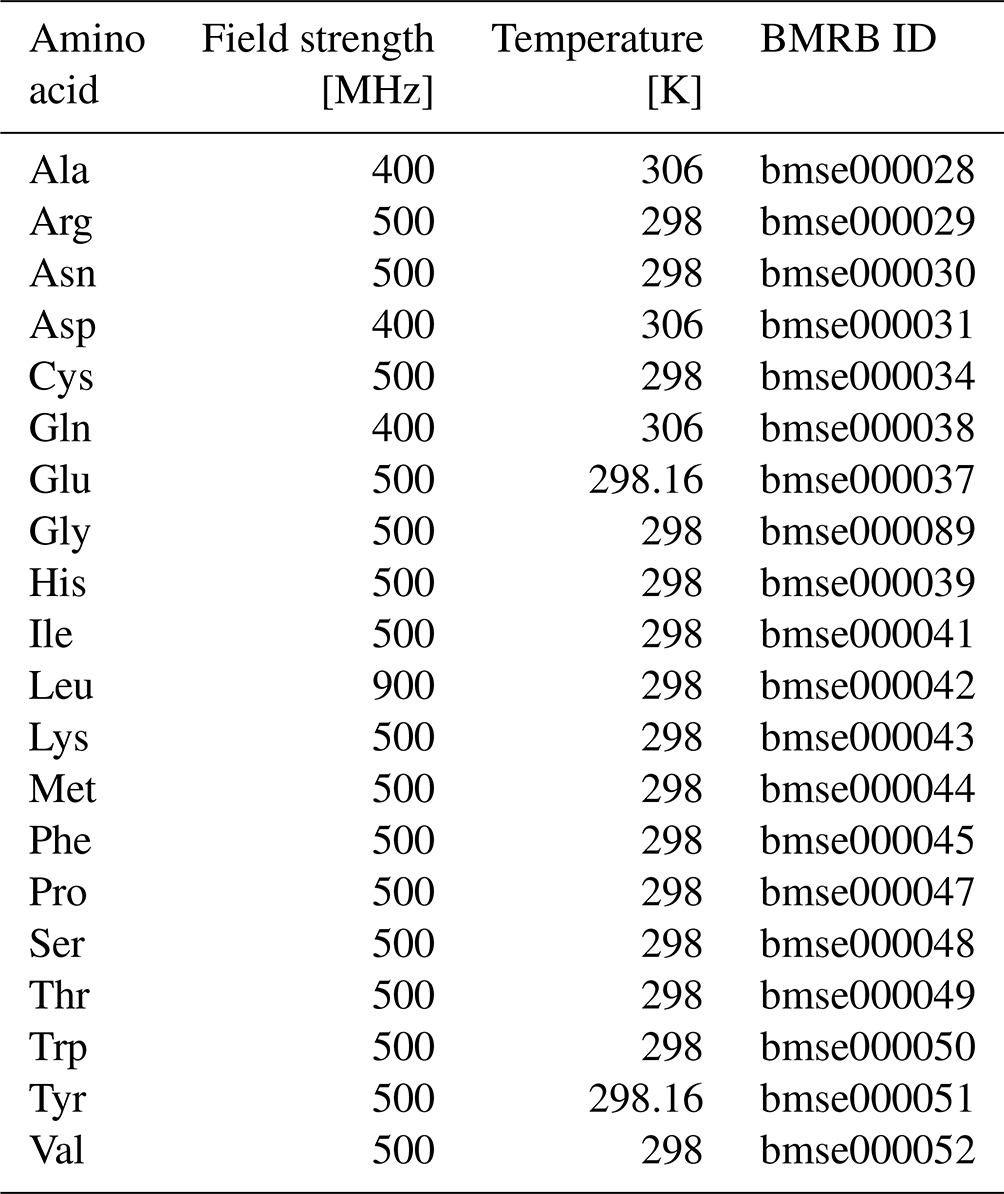
Table A2Generalized Karplus equation parameters for 1H-1H 3J couplings. gives the difference in substituent group electronegativity.
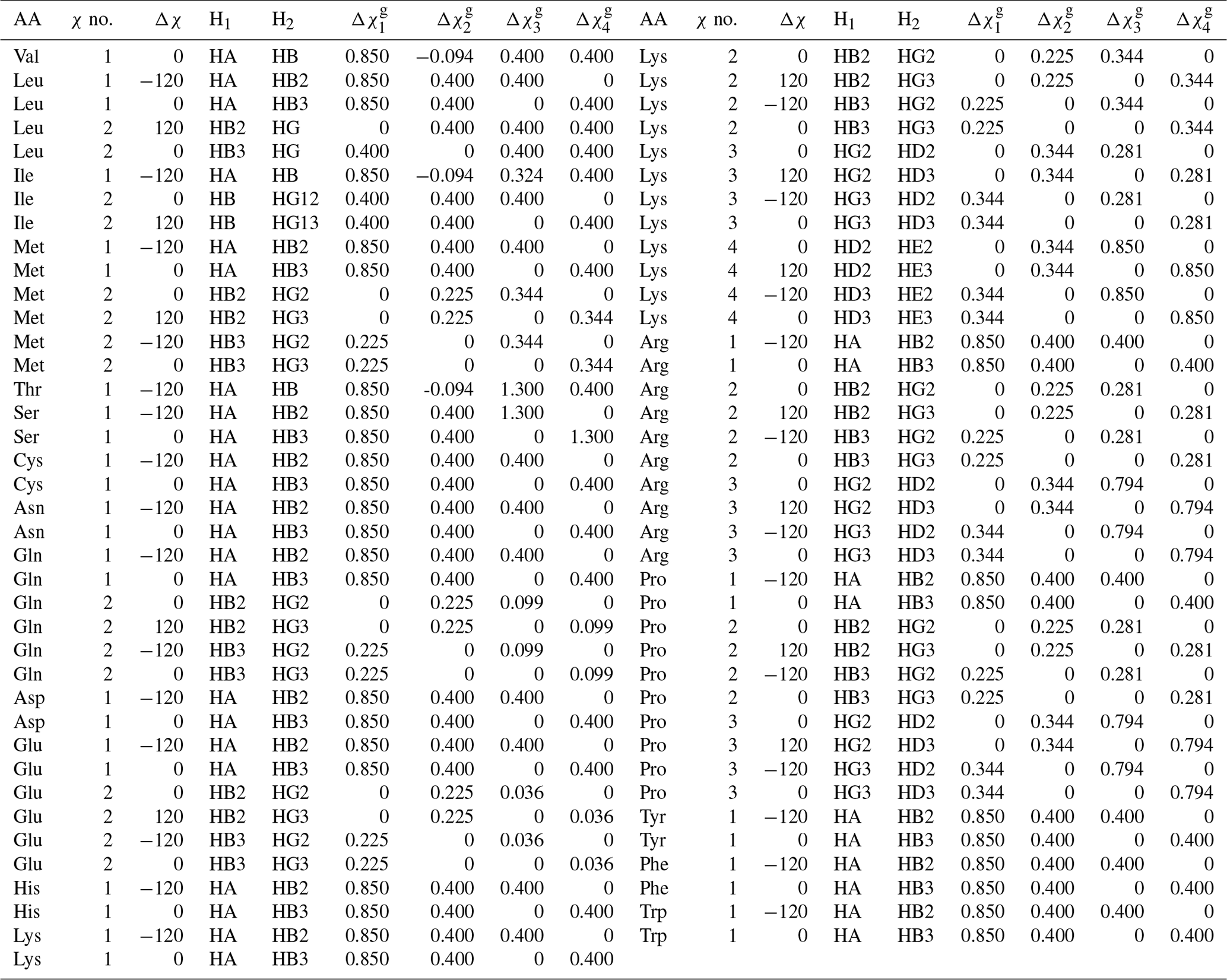
Table A3Self-consistent Karplus equation parameters for 1H–1H 3J couplings. Ni gives the number of each type of substituent heavy atom.
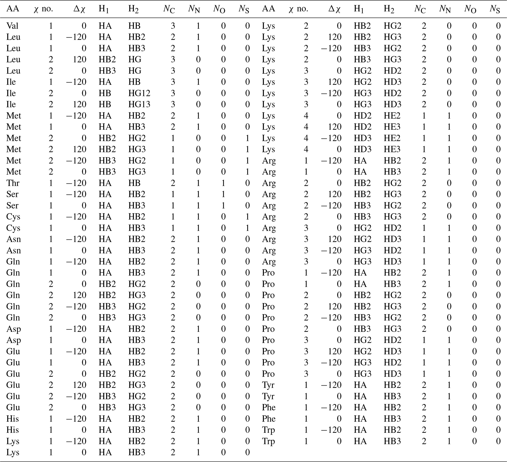
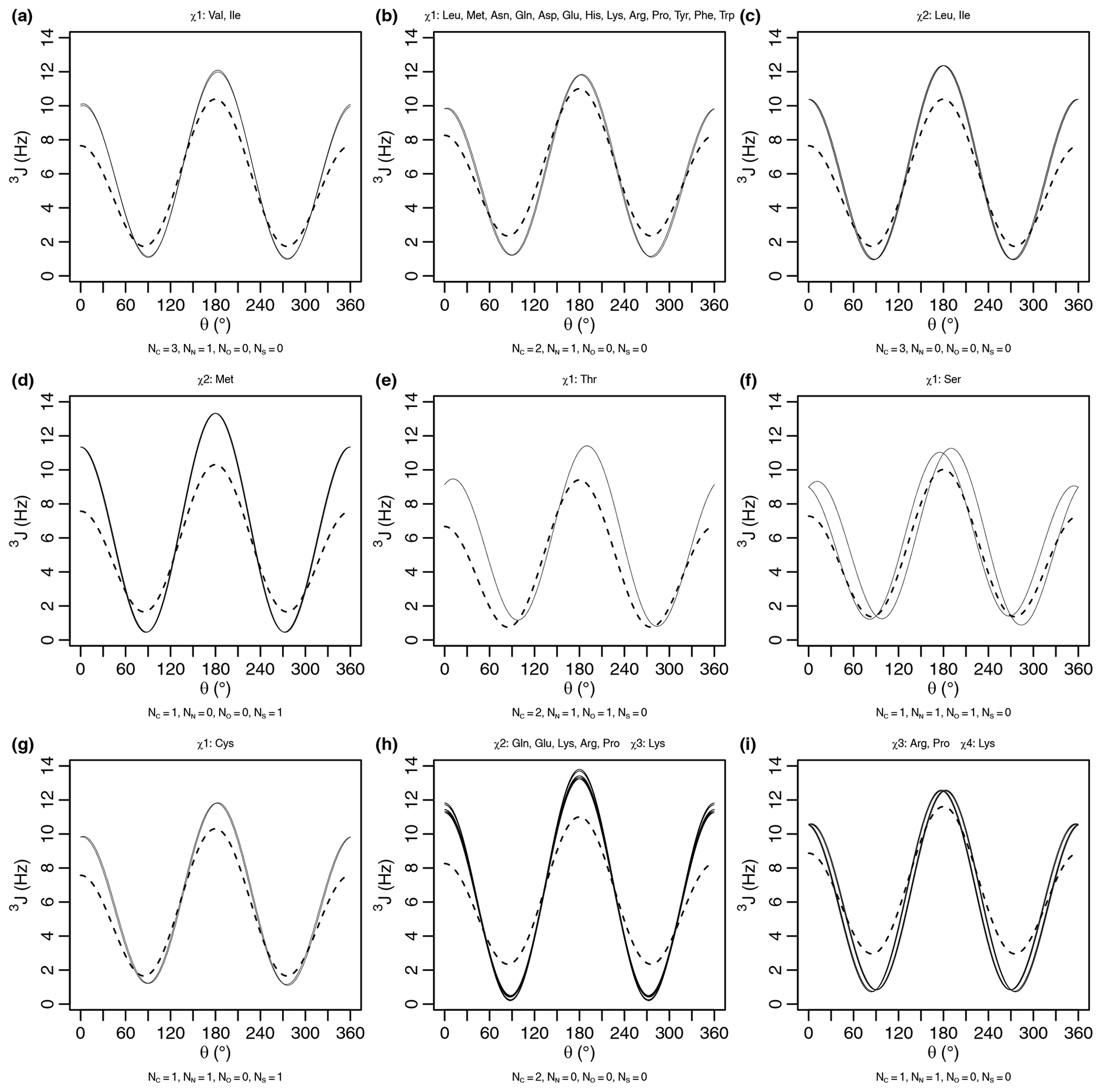
Figure A1Generalized Karplus equation (thin lines) and self-consistent Karplus equation (dashed lines) for proton–proton 3J scalar couplings across different χ angles. The number of atoms (Ni) used for generating the self-consistent Karplus curves is given as a subtitle. The generalized Karplus curve phase shifts observed in (f) and (i) come from large differences in the electronegativity between substituents 3 and 4 (see Table A2).
This paper was prepared using R Markdown. All code and data required for reproducing the paper, figures, and tables in their entirety are available in the Supplement distributed with the paper. See the README.md file within for more details. The Supplement is also available at https://github.com/smith-group/syed2024 (Syed et al., 2024), which may be updated as necessary to maintain software compatibility. The fitting methodology is implemented in the FitNMR open-source R package at https://github.com/smith-group/fitnmr (Smith and Dudley, 2024).
The supplement related to this article is available online at: https://doi.org/10.5194/mr-5-103-2024-supplement.
NRS and NBM carried out fits of the one-dimensional NMR spectra. CAS carried out the other analyses and wrote the paper.
The contact author has declared that none of the authors has any competing interests.
Publisher’s note: Copernicus Publications remains neutral with regard to jurisdictional claims made in the text, published maps, institutional affiliations, or any other geographical representation in this paper. While Copernicus Publications makes every effort to include appropriate place names, the final responsibility lies with the authors.
This research has been supported by the National Institutes of Health (grant no. 1R15GM141974-01).
This paper was edited by Nicola Salvi and reviewed by two anonymous referees.
Achanta, P. S., Jaki, B. U., McAlpine, J. B., Friesen, J. B., Niemitz, M., Chen, S.-N., and Pauli, G. F.: Quantum mechanical NMR full spin analysis in pharmaceutical identity testing and quality control, J. Pharmaceut. Biomed., 192, 113601, https://doi.org/10.1016/j.jpba.2020.113601, 2021. a
Ahlner, A., Carlsson, M., Jonsson, B.-H., and Lundström, P.: PINT: a software for integration of peak volumes and extraction of relaxation rates, J. Biomol. NMR, 56, 191–202, https://doi.org/10.1007/s10858-013-9737-7, 2013. a
Bernstein, M. A., Sýkora, S., Peng, C., Barba, A., and Cobas, C.: Optimization and Automation of Quantitative NMR Data Extraction, Anal. Chem., 85, 5778–5786, https://doi.org/10.1021/ac400411q, 2013. a
Bundi, A. and Wüthrich, K.: 1H-nmr parameters of the common amino acid residues measured in aqueous solutions of the linear tetrapeptides H-Gly-Gly-X-L-Ala-OH, Biopolymers, 18, 285–297, https://doi.org/10.1002/bip.1979.360180206, 1979. a, b
Cao, L., Coventry, B., Goreshnik, I., Huang, B., Sheffler, W., Park, J. S., Jude, K. M., Marković, I., Kadam, R. U., Verschueren, K. H. G., Verstraete, K., Walsh, S. T. R., Bennett, N., Phal, A., Yang, A., Kozodoy, L., DeWitt, M., Picton, L., Miller, L., Strauch, E.-M., DeBouver, N. D., Pires, A., Bera, A. K., Halabiya, S., Hammerson, B., Yang, W., Bernard, S., Stewart, L., Wilson, I. A., Ruohola-Baker, H., Schlessinger, J., Lee, S., Savvides, S. N., Garcia, K. C., and Baker, D.: Design of protein-binding proteins from the target structure alone, Nature, 605, 551–560, https://doi.org/10.1038/s41586-022-04654-9, 2022. a
Castellano, S. and Bothner‐By, A. A.: Analysis of NMR Spectra by Least Squares, J. Chem. Phys., 41, 3863–3869, https://doi.org/10.1063/1.1725826, 1964. a
Castillo, A. M., Patiny, L., and Wist, J.: Fast and accurate algorithm for the simulation of NMR spectra of large spin systems, J. Magn. Reson., 209, 123–130, https://doi.org/10.1016/j.jmr.2010.12.008, 2011. a
Cheshkov, D. A. and Sinitsyn, D. O.: Chapter Two – Total line shape analysis of high-resolution NMR spectra, Vol. 100, 61–96, Academic Press, ISBN 0066-4103, https://doi.org/10.1016/bs.arnmr.2019.11.001, 2020. a
Cheshkov, D. A., Sheberstov, K. F., Sinitsyn, D. O., and Chertkov, V. A.: ANATOLIA: NMR software for spectral analysis of total lineshape, Magn. Reson. Chem., 56, 449–457, https://doi.org/10.1002/mrc.4689, 2018. a
Dashti, H., Westler, W. M., Tonelli, M., Wedell, J. R., Markley, J. L., and Eghbalnia, H. R.: Spin System Modeling of Nuclear Magnetic Resonance Spectra for Applications in Metabolomics and Small Molecule Screening, Anal. Chem., 89, 12201–12208, https://doi.org/10.1021/acs.analchem.7b02884, 2017. a, b
Dashti, H., Wedell, J. R., Westler, W. M., Tonelli, M., Aceti, D., Amarasinghe, G. K., Markley, J. L., and Eghbalnia, H. R.: Applications of Parametrized NMR Spin Systems of Small Molecules, Anal. Chem., 90, 10646–10649, https://doi.org/10.1021/acs.analchem.8b02660, 2018. a, b
Delaglio, F., Grzesiek, S., Vuister, G. W., Zhu, G., Pfeifer, J., and Bax, A.: NMRPipe: A multidimensional spectral processing system based on UNIX pipes, J. Biomol. NMR, 6, 277–293, https://doi.org/10.1007/BF00197809, 1995. a
Delaglio, F., Wu, Z., and Bax, A.: Measurement of Homonuclear Proton Couplings from Regular 2D COSY Spectra, J. Magn. Reson., 149, 276–281, https://doi.org/10.1006/jmre.2001.2297, 2001. a, b
Dudley, J. A., Park, S., MacDonald, M. E., Fetene, E., and Smith, C. A.: Resolving overlapped signals with automated FitNMR analytical peak modeling, J. Magn. Reson., 318, 106773, https://doi.org/10.1016/j.jmr.2020.106773, 2020. a, b, c
Dudley, J. A., Park, S., Cho, O., Wells, N. G. M., MacDonald, M. E., Blejec, K. M., Fetene, E., Zanderigo, E., Houliston, S., Liddle, J. C., Dashnaw, C. M., Sabo, T. M., Shaw, B. F., Balsbaugh, J. L., Rocklin, G. J., and Smith, C. A.: Heat-induced structural and chemical changes to a computationally designed miniprotein, Protein Sci., 33, e4991, https://doi.org/10.1002/pro.4991, 2024. a, b
Dzakula, Z., Edison, A. S., Westler, W. M., and Markley, J. L.: Analysis of chi1 rotamer populations from NMR data by the CUPID method, J. Am. Chem. Soc., 114, 6200–6207, https://doi.org/10.1021/ja00041a044, 1992. a
Emerson, S. D. and Montelione, G. T.: 2D and 3D HCCH TOCSY experiments for determining 3J(HαHβ) coupling constants of amino acid residues, J. Magn. Reson., 99, 413–420, https://doi.org/10.1016/0022-2364(92)90196-E, 1992. a
Gemmecker, G. and Fesik, S. W.: A method for measuring 1H-1H coupling constants in 13C-labeled molecules, J. Magn. Reson., 95, 208–213, https://doi.org/10.1016/0022-2364(91)90340-Y, 1991. a
Griesinger, C. and Eggenberger, U.: Determination of proton-proton coupling constants in 13C-labeled molecules, J. Magn. Reson., 97, 426–434, https://doi.org/10.1016/0022-2364(92)90328-5, 1992. a
Griesinger, C., Sørensen, O. W., and Ernst, R. R.: Two-dimensional correlation of connected NMR transitions, J. Am. Chem. Soc., 107, 6394–6396, https://doi.org/10.1021/ja00308a042, 1985. a
Griesinger, C., Sørensen, O. W., and Ernst, R. R.: Correlation of connected transitions by two‐dimensional NMR spectroscopy, J. Chem. Phys., 85, 6837–6852, https://doi.org/10.1063/1.451421, 1986. a
Griesinger, C., Sørensen, O. W., and Ernst, R. R.: Practical aspects of the E.COSY technique. Measurement of scalar spin-spin coupling constants in peptides, J. Magn. Reson., 75, 474–492, https://doi.org/10.1016/0022-2364(87)90102-8, 1987. a
Grzesiek, S., Kuboniwa, H., Hinck, A. P., and Bax, A.: Multiple-Quantum Line Narrowing for Measurement of Hα-Hβ J Couplings in Isotopically Enriched Proteins, J. Am. Chem. Soc., 117, 5312–5315, https://doi.org/10.1021/ja00124a014, 1995. a
Haasnoot, C. A. G., de Leeuw, F. A. A. M., de Leeuw, H. P. M., and Altona, C.: Interpretation of vicinal proton-proton coupling constants by a generalized Karplus relation. Conformational analysis of the exocyclic C4'-C5' bond in nucleosides and nucleotides: Preliminary Communication, Recl. Trav. Chim. Pay.-B, 98, 576–577, https://doi.org/10.1002/recl.19790981206, 1979. a
Haasnoot, C. A. G., de Leeuw, F. A. A. M., and Altona, C.: The relationship between proton-proton NMR coupling constants and substituent electronegativities – I: An empirical generalization of the karplus equation, Tetrahedron, 36, 2783–2792, https://doi.org/10.1016/0040-4020(80)80155-4, 1980. a, b, c, d, e, f, g, h
Haasnoot, C. A. G., de Leeuw, F. A. A. M., de Leeuw, H. P. M., and Altona, C.: The relationship between proton–proton NMR coupling constants and substituent electronegativities. II – conformational analysis of the sugar ring in nucleosides and nucleotides in solution using a generalized Karplus equation, Org. Magn. Resonance, 15, 43–52, https://doi.org/10.1002/mrc.1270150111, 1981a. a
Haasnoot, C. A. G., De Leeuw, F. A. A. M., De Leeuw, H. P. M., and Altona, C.: Relationship between proton–proton nmr coupling constants and substituent electronegativities. III. Conformational analysis of proline rings in solution using a generalized Karplus equation, Biopolymers, 20, 1211–1245, https://doi.org/10.1002/bip.1981.360200610, 1981b. a, b
Heinzer, J.: Iterative least-squares nmr lineshape fitting with use of symmetry and magnetic equivalence factorization, J. Magn. Reson., 26, 301–316, https://doi.org/10.1016/0022-2364(77)90176-7, 1977. a
Hoch, J. C., Baskaran, K., Burr, H., Chin, J., Eghbalnia, H. R., Fujiwara, T., Gryk, M. R., Iwata, T., Kojima, C., Kurisu, G., Maziuk, D., Miyanoiri, Y., Wedell, J. R., Wilburn, C., Yao, H., and Yokochi, M.: Biological Magnetic Resonance Data Bank, Nucleic Acids Res., 51, D368–D376, https://doi.org/10.1093/nar/gkac1050, 2023. a
Hogben, H. J., Krzystyniak, M., Charnock, G. T. P., Hore, P. J., and Kuprov, I.: Spinach – A software library for simulation of spin dynamics in large spin systems, J. Magn. Reson., 208, 179–194, https://doi.org/10.1016/j.jmr.2010.11.008, 2011. a
Huber, P., Zwahlen, C., Vincent, S. J. F., and Bodenhausen, G.: Accurate Determination of Scalar Couplings by Convolution of Complementary Two-Dimensional Multiplets, J. Magn. Reson. Ser. A, 103, 118–121, https://doi.org/10.1006/jmra.1993.1142, 1993. a, b
Huggins, M. L.: Bond Energies and Polarities, J. Am. Chem. Soc., 75, 4123–4126, https://doi.org/10.1021/ja01113a001, 1953. a
Inagaki, F.: Protein NMR Resonance Assignment, 2033–2037, Springer Berlin Heidelberg, Berlin, Heidelberg, ISBN 978-3-642-16712-6, https://doi.org/10.1007/978-3-642-16712-6_312, 2013. a
Karplus, M.: Vicinal Proton Coupling in Nuclear Magnetic Resonance, J. Am. Chem. Soc., 85, 2870–2871, https://doi.org/10.1021/ja00901a059, 1963. a, b
Kessler, H., Müller, A., and Oschkinat, H.: Differences and sums of traces within, COSY spectra (DISCO) for the extraction of coupling constants: “Decoupling” after the measurement, Magn. Reson. Chem., 23, 844–852, https://doi.org/10.1002/mrc.1260231012, 1985. a, b
Kraszni, M., Szakács, Z., and Noszál, B.: Determination of rotamer populations and related parameters from NMR coupling constants: a critical review, Anal. Bioanal. Chem., 378, 1449–1463, https://doi.org/10.1007/s00216-003-2386-z, 2004. a
Li, D.-W., Bruschweiler-Li, L., Hansen, A. L., and Brüschweiler, R.: DEEP Picker1D and Voigt Fitter1D: a versatile tool set for the automated quantitative spectral deconvolution of complex 1D-NMR spectra, Magn. Reson., 4, 19–26, https://doi.org/10.5194/mr-4-19-2023, 2023. a
Li, F., Grishaev, A., Ying, J., and Bax, A.: Side Chain Conformational Distributions of a Small Protein Derived from Model-Free Analysis of a Large Set of Residual Dipolar Couplings, J. Am. Chem. Soc., 137, 14798–14811, https://doi.org/10.1021/jacs.5b10072, 2015. a
Löhr, F., Schmidt, J. M., and Rüterjans, H.: Simultaneous Measurement of 3JHN,Hα and 3JHα,Hβ Coupling Constants in 13C,15N-Labeled Proteins, J. Am. Chem. Soc., 121, 11821–11826, https://doi.org/10.1021/ja991356h, 1999. a
Mittermaier, A. and Kay, L. E.: χ1 Torsion Angle Dynamics in Proteins from Dipolar Couplings, J. Am. Chem. Soc., 123, 6892–6903, https://doi.org/10.1021/ja010595d, 2001. a
Niklasson, M., Otten, R., Ahlner, A., Andresen, C., Schlagnitweit, J., Petzold, K., and Lundström, P.: Comprehensive analysis of NMR data using advanced line shape fitting, J. Biomol. NMR, 69, 93–99, https://doi.org/10.1007/s10858-017-0141-6, 2017. a
Oschkinat, H. and Freeman, R.: Fine structure in two-dimensional NMR correlation spectroscopy, J. Magn. Reson., 60, 164–169, https://doi.org/10.1016/0022-2364(84)90044-1, 1984. a, b
Pachler, K. G. R.: Nuclear magnetic resonance study of some α-amino acids – I: Coupling constants in alkaline and acidic medium, Spectrochim. Acta, 19, 2085–2092, https://doi.org/10.1016/0371-1951(63)80228-3, 1963. a
Pérez, C., Löhr, F., Rüterjans, H., and Schmidt, J. M.: Self-consistent Karplus parametrization of 3J couplings depending on the polypeptide side-chain torsion χ1, J. Am. Chem. Soc., 123, 7081–7093, https://doi.org/10.1021/ja003724j, 2001. a, b, c, d, e, f, g, h, i
Prasch, T., Gröschke, P., and Glaser, S. J.: SIAM, a Novel NMR Experiment for the Determination of Homonuclear Coupling Constants, Angew. Chem. Int. Edit., 37, 802–806, https://doi.org/10.1002/(SICI)1521-3773(19980403)37:6<802::AID-ANIE802>3.0.CO;2-M, 1998. a, b
Schmidt, J. M., Blümel, M., Löhr, F., and Rüterjans, H.: Self-consistent 3J coupling analysis for the joint calibration of Karplus coefficients and evaluation of torsion angles, J. Biomol. NMR, 14, 1–12, https://doi.org/10.1023/A:1008345303942, 1999. a, b, c
Shapovalov, M. V. and Dunbrack, R. L.: A Smoothed Backbone-Dependent Rotamer Library for Proteins Derived from Adaptive Kernel Density Estimates and Regressions, Structure, 19, 844–858, https://doi.org/10.1016/j.str.2011.03.019, 2011. a
Smith, A. A.: INFOS: spectrum fitting software for NMR analysis, J. Biomol. NMR, 67, 77–94, https://doi.org/10.1007/s10858-016-0085-2, 2017. a
Smith, C. A. and Dudley, J.: Smith-Group/fitnmr, GitHub [code], https://github.com/smith-group/fitnmr, last access: 10 August 2024. a
Smith, L. J., van Gunsteren, W. F., Stankiewicz, B., and Hansen, N.: On the use of 3J-coupling NMR data to derive structural information on proteins, J. Biomol. NMR, 75, 39–70, https://doi.org/10.1007/s10858-020-00355-5, 2021. a
Steiner, D., Allison, J. R., Eichenberger, A. P., and van Gunsteren, W. F.: On the calculation of 3Jαβ-coupling constants for side chains in proteins, J. Biomol. NMR, 53, 223–246, https://doi.org/10.1007/s10858-012-9634-5, 2012. a
Syed, N. R., Masud, N. B., and Smith, C. A.: Smith-Group/syed2024, GitHub [code, data set], https://github.com/smith-group/syed2024, last access: 10 August 2024. a
Tessari, M., Mariani, M., Boelens, R., and Kaptein, R.: (H)XYH-COSY and (H)XYH-E.COSY Experiments for Backbone and Side-Chain Assignment and Determination of Coupling Constants in (13C, 15N)-Labeled Proteins, J. Magn. Reson. Ser. B, 108, 89–93, https://doi.org/10.1006/jmrb.1995.1108, 1995. a
Tiainen, M., Soininen, P., and Laatikainen, R.: Quantitative Quantum Mechanical Spectral Analysis (qQMSA) of 1H NMR spectra of complex mixtures and biofluids, J. Magn. Reson., 242, 67–78, https://doi.org/10.1016/j.jmr.2014.02.008, 2014. a
Titman, J. J. and Keeler, J.: Measurement of homonuclear coupling constants from NMR correlation spectra, J. Magn. Reson., 89, 640–646, https://doi.org/10.1016/0022-2364(90)90351-9, 1990. a, b
Veshtort, M. and Griffin, R. G.: SPINEVOLUTION: A powerful tool for the simulation of solid and liquid state NMR experiments, J. Magn. Reson., 178, 248–282, https://doi.org/10.1016/j.jmr.2005.07.018, 2006. a
Vuister, G. W. and Bax, A.: Quantitative J correlation: a new approach for measuring homonuclear three-bond J(HNHα) coupling constants in 15N-enriched proteins, J. Am. Chem. Soc., 115, 7772–7777, https://doi.org/10.1021/ja00070a024, 1993. a
Vuister, G. W., Tessari, M., Karimi-Nejad, Y., and Whitehead, B.: Pulse Sequences for Measuring Coupling Constants, 195–257, Springer US, Boston, MA, ISBN 978-0-306-47083-7, https://doi.org/10.1007/0-306-47083-7_6, 2002. a
Westbrook, J. D., Shao, C., Feng, Z., Zhuravleva, M., Velankar, S., and Young, J.: The chemical component dictionary: complete descriptions of constituent molecules in experimentally determined 3D macromolecules in the Protein Data Bank, Bioinformatics, 31, 1274–1278, https://doi.org/10.1093/bioinformatics/btu789, 2015. a
Wüthrich, K.: NMR of proteins and nucleic acids, Wiley, New York, ISBN 0471828939, 1986. a