the Creative Commons Attribution 4.0 License.
the Creative Commons Attribution 4.0 License.
 | 09 Feb 2022
Spin relaxation: is there anything new under the Sun?
Bogdan A. Rodin
Spin relaxation has been at the core of many studies since the early days of nuclear magnetic resonance (NMR) and the underlying theory worked out by its founding fathers. This Bloch–Redfield–Abraham relaxation theory has been recently reinvestigated (Bengs and Levitt, 2020) in the perspective of Lindblad theory of quantum Markovian master equations in order to account for situations where the widely used semi-classical relaxation theory breaks down. In this article, we review the conventional approach of quantum mechanical theory of NMR relaxation and show that, under the usual assumptions, it is equivalent to the Lindblad formulation. We also comment on the debate on semi-classical versus quantum versions of spectral density functions involved in relaxation.
- Article
(734 KB) - Full-text XML
- BibTeX
- EndNote


Relaxation is the process through which a system loses energy to its environment to eventually reach a state of thermal equilibrium. Spin–lattice relaxation has been described as the way spins transfer energy to orientation degrees of freedom. Since the early days of nuclear magnetic resonance (NMR), it has been the subject of numerous studies, both theoretical and encompassing a wide range of domains of applications. NMR relaxation theory really was contemporary in the early days of NMR, and it was formalized by several of its founding fathers (Bloembergen et al., 1948; Bloch, 1957, 1956; Abragam, 1961; Redfield, 1957, 1965). This is a rather usual approach to the theory of open systems, which has been widely used in various domains of physics (VanKampen, 1981). From this perspective, relaxation is the result of the dynamical coupling of a small ensemble of spins (the system) coupled to a large ensemble of particles, or degrees of freedom (the lattice), that are at thermal (Boltzmann) equilibrium and are endowed with an infinite heat capacity, thereby constituting a thermal reservoir. This very general approach has led to many theoretical predictions with far-reaching practical applications in the domain of magnetic resonance spectroscopy. In particular, the role played by molecular motions has been put to good use to extract dynamical information on complex molecular objects. Thus, with the development of spin engineering techniques, it has become possible to measure selected relaxation rates with high accuracy in a broad range of problems, with the prospect of relating such observables to models of molecular dynamics.
It has been shown recently by Bengs and Levitt (2020) that the formulation of Redfield's semi-classical theory of relaxation widely used by NMR spectroscopists may lead to erroneous predictions in the case of a two-spin system prepared in high-order states, such as singlet spin states.
Such an unexpected behavior was ascribed to the fact that some of the assumptions of the theory may not be fulfilled in NMR systems, and the authors solved the problem by making use of the Lindblad operator, which is commonly used in the theory of open quantum systems to account for dissipative Markovian phenomena, i.e., relaxation processes. Among other properties, the structure of the Lindblad operator ensures that the fundamental properties of the density operator ρ (ρ, which is hermitian and definite positive, and Tr(ρ)=1) are preserved (Lindblad, 1976; Alicki and Lendi, 2007). This article has sparked renewed interest regarding the general theory of relaxation, as first elaborated by Bloch, and its connection with the Lindblad theory of quantum dissipative systems (Barbara, 2021). This approach has been generalized in several recent works (Nathan and Rudner, 2020; Maimbourg et al., 2021).
The traditional description of NMR relaxation relies on the description of both the spin system and the lattice as quantum systems, an approach that leads to the celebrated Redfield equation (Bloch, 1956; Redfield, 1965; Hubbard, 1961; see also Goldman, 2001, for a more recent account on spin lattice relaxation). As far as the description of the lattice is concerned, this approach is challenging, and actually untractable, as a quantized description of the degrees of freedom involved in molecular motions (multiple bond rotations, overall tumbling of a molecule, etc.) is not manageable in practice, even for small molecular systems. For this reason, an alternative relaxation theory, where the spins are treated as quantum objects and the lattice is described with classical functions of the lattice degrees of freedom, was developed. This semi-classical approach has far-reaching practical consequences, as spin relaxation can then, in principle, be described using classical models of dynamics for molecular motions, and it has been extensively used over the years to describe and interpret spin relaxation experiments. However, this semi-classical theory predicts a non-Boltzmann equilibrium density operator, which requires an ad hoc thermal correction to the relaxation equations (Redfield, 1965; Abragam, 1961). More elaborate attempts have been made to overcome this limitation by modifying the relaxation operator itself and to enforce a Boltzmann equilibrium of the density operator (Jeener, 1982; Levitt and Bari, 1992). However, in the traditional semi-classical NMR relaxation approach and its later modifications, the spin–lattice interactions are accounted for by a stochastic, fluctuating Hamiltonian. This has important consequences. First, in the conventional Abraham–Redfield approach, the statistical properties of the (classical) lattice are not constrained by a fluctuation–dissipation kind of theorem that would enforce a Boltzmann equilibrium distribution and, therefore, a lattice temperature. Such a constraint is therefore not applied on the spins. Second, a major difference between the quantum and classical theories of spin relaxation is rooted in the non-commutation of quantum bath operators of the spin–lattice coupling Hamiltonian, which confers particular properties to the spin correlation and spectral density functions that are absent in the semi-classical theory. Both aspects, quantum and statistical, are entangled, and the relations between quantum and classical correlation functions will therefore be discussed.
It is the purpose of this paper to re-investigate these old questions in order to trace the roles and the consequences of the various assumptions of the traditional approach to relaxation developed in the early days of NMR.
2.1 Derivation of the master equation
The derivation follows the lines of Abragam (1961), Bloch (1956), Redfield (1957), and Hubbard (1961). Consider a spin system in its environment. The Hamiltonian of the spin system HS accounts for the interaction of the spins with the magnetic fields (Zeeman interaction and interaction with a radio frequency (rf) field) and non-dissipative spin–spin interactions (scalar J coupling and dipolar coupling). The dynamics of the lattice (the bath) are described by HB, and the spin–bath interaction Hamiltonian is H1, as follows:
and the dynamics of the {spin–bath} system are described by the Liouville equation as follows:
Alternatively, it can be written as follows:
where the operator is the total Liouvillian. Introducing the density operator in the interaction representation of the density operator , where is the unperturbed Liouvillian, one has the following:
The Liouville equation is integrated to the second order as follows:
Taking the derivative, one obtains the following:
Finally, by making the change in the variables , one obtains the master equation for the total density operator as follows:
The dynamics restricted to the spin system are obtained by eliminating the bath variables. This is achieved by performing a partial trace over the bath degrees of freedom as follows:
Hence, from Eq. (6), the spin density operator in the interaction representation is as follows:
which obeys the following:
Initially, the system and the bath are assumed to be completely decorrelated, as follows:
where the exact denotes the bath density operator in thermal equilibrium. With these assumptions, one has the following:
In the latter expression, the term may be assumed to be zero or can be incorporated in the main system Liouvillian ℒS as follows (Abragam, 1961; Redfield, 1957):
If the spin density operator is assumed to only moderately depart from its initial state, then the following occurs:
where the density operator varies only slightly from its initial state so that σ∗(0) can be replaced by σ∗(t) in Eq. (12), as follows (Abragam, 1961; Redfield, 1957):
The master equation in the Schrödinger representation can be obtained from Eq. (15) as follows:
Therefore, one has the following:
Reverting to the Schrödinger representation , one obtains the following master equation in the Schrödinger representation:
A derivation is given in Appendix A for reference. The term in Eq. (18) is a correlation operator acting on the spin system. It projects the system–bath (spin–lattice) coupling onto the bath degrees of freedom. This spin operator therefore carries the statistical properties of the bath, described by its equilibrium and stationary density operator. Finally, assuming that the correlation operator decays to zero in a time τc much shorter than the period over which the density matrix varies significantly, the upper limit of the integral can be extended to +∞. As above, making the change in the variables , one obtains the following:
or, in the following Hamiltonian representation, the following:
One, therefore, obtains a master equation of the Redfield kind, as follows:
where is the Redfield (relaxation) operator.
2.2 Formulation of the master equation in operator form
In spin relaxation theory, it is customary to express the relaxation equation in the operator form, which often provides a clearer representation of the spin–bath coupling dynamics. Here, the coupling Hamiltonian is assumed to have the form of a sum of terms, each of which factorizes into a product of lattice Bq and spin Sq operators.
with the interaction representation as follows:
Using results of the preceding section (Eqs. 16–18), the Redfield equation becomes the following:
Each term in the sum becomes the following:
where the notation, as in the following:
has been introduced. The are the bath (lattice) correlation functions, and in contrast to Eq. (19), these denote usual time correlation functions rather than operators.
Using the conventional decomposition of the spin operators into a sum of eigenoperators of the Liouvillian as follows:
one has the following:
which one obtains from Eq. (28), with the change in the integration variable as follows:
Introducing the secular approximation , so that , and renaming the indices reduces to the following:
The assumption that the bath is in a stationary state, , confers some properties to the correlation functions. Thus, the bath correlation functions are also stationary. Indeed, one has the following:
In addition, because , it is easy to show the following:
Besides, using the property that , as in the following:
where the |f〉 are the eigenstates of the bath Hamiltonian, HB, and , with the convention ℏ=1. In these equation, the notation was introduced.
It is now straightforward to show that the conventional Bloch–Redfield–Abraham perturbative approach of relaxation is equivalent to the Lindblad formulation of dissipative systems. Indeed, by changing indices in the first term, using the property , and setting , one has, from Eq. (32), the following:
Using the stationarity property (Eq. 33) of the bath correlation functions leads to following:
so that, in the following:
where the right spectral density of the bath is given by the following:
where denotes the anti-commutator. The operator appearing on the right-hand side of Eq. (39) is the Lindblad dissipation super-operator, as follows:
so that Eq. (39) becomes the following:
Equation (42) (and Eq. 39) is a Lindblad equation (Lindblad, 1976; Alicki and Lendi, 2007), which is thus derived from the usual quantized theory of relaxation (Bloch, 1957; Redfield, 1957; Hubbard, 1961; Abragam, 1961).
The fact that this derivation leads to the Lindblad equation is not obvious. In principle, one should not expect the perturbative approach to yield an irreversible dissipative operator equivalent to a Lindblad operator. In fact, this equivalence requires the Markovian and the short correlation time assumptions that make the evolution equation depend on the density operator at the present time t only and not in its previous history. Moreover, it also requires the secular approximation that eliminates the time dependence of the spin operators of the coupling Hamiltonian in Eq. (28), leading to Eq. (32). The combination of these conditions lead to the semi-group property and the Lindblad form of the relaxation operator.
Another point is worth mentioning. The properties of the correlation functions that emerge through this procedure reflect the properties of the bath operators of the spin–bath coupling Hamiltonian and, therefore, convey additional properties that are not implied by the structure of the Lindblad in Eqs. (39) and (42). Such properties, arising from the non-commutation of the bath operators and the fact that the lattice is always in a stationary Boltzmann equilibrium (detailed in Sect. 3.1 below and in Appendix B), ensure a detailed balance and that the stationary state of the spin system is compatible with the Boltzmann equilibrium of the lattice, that is, the lattice temperature. In other words, the perturbative approach leads to a master equation of the Lindblad form, with additional physical properties that bear constraints from the lattice.
3.1 An alternative formulation (equivalent to Lindblad)
It is possible to obtain an alternative and completely equivalent form of the Redfield equation. Expanding Eq. (32), one obtains the following:
As above, the left-hand side spectral density function is defined as follows:
where (ℏ=1). The latter equations express a Kubo kind of relation (Kubo, 1957), where . A proof thereof is given in the Appendix (see Eqs. B1 and B3). After some straightforward manipulations, one obtains the following:
Thus, by collecting and rearranging terms, one obtains the following:
The Boltzmann factor can be expanded in a series, as follows:
The first term on the right-hand side of this equation is the usual double commutator and the symmetry, while the second term represents the thermal effect of the Boltzmann equilibrium of the lattice. This term, equal to , vanishes for infinite temperature.
A semi-classical version of the master equation can be extremely useful, allowing one to make use of models derived from the framework of classical mechanics to calculate the spectral density functions. In order to obtain such a theory associated to Eqs. (39) and (42), additional adjustments are necessary. Indeed, because the B−q(τ) operators do not commute, the correlation functions of the type 〈B−q(τ)Bq〉 do not obey the general symmetry rules of classical correlation functions. However, symmetrized correlation functions do commute, and so these symmetrized (quantum mechanical) correlation functions should be introduced in order to obtain a semi-classical theory (which we call pseudo-classical to distinguish it from the theory where the effect of the bath is taken into account only through random functions). A general definition of the classical correlation function of two dynamical variables A and B is as follows (Evans and Moriss, 2008):
where the brackets indicate classical ensemble average. In the case of stationary processes, the following properties of a correlation function can be deduced. Its complex conjugate is, therefore, as follows (Evans and Moriss, 2008):
For an autocorrelation function of A and CAA(t), one has the following:
Equation (50) shows that, in the general case where the autocorrelation function is complex, , with and are even and odd functions of time, since . This implies that the associated spectral density, is real and , , and are real and, respectively, even and odd functions.
A semi-classical relaxation theory should provide spectral density functions obeying the general classical mechanics requirements detailed above. It is clear, however, that in the quantum case, where A and B are in general non-commuting operators, the above symmetry relations do no apply. It is nevertheless possible to define a symmetrized correlation function as follows:
which is real when CAB(t) is stationary. Note also that the bath operator correlation functions have the following property:
where correlation functions are assumed stationary, so that, in the following:
Using the definitions and , the relations in Eqs. (53) and (54) show that the average obey the classical correlation function property .
A semi-classical version of the Redfield equation is thus obtained by using the spectral density function Jq(ω) obtained from the Fourier transform of the symmetrized correlation function Cq(τ), as follows:
Using Eqs. (55) and (45), it is therefore possible to derive an alternative expression of the master equation. This gives the following:
or the following:
Finally, from collecting and rearranging terms, one obtains the following:
In view of clarifying the connection between the derivation of the quantum mechanical master equation to further semi-classical approximations, it is interesting to rewrite Eq. (58) by expanding the temperature function in terms of the parameters , as follows:
Equation (59) contains a double commutator term weighted by the spectral densities , which are constructed so as to obey the general symmetry properties of classical spectral density functions (see Eq. 48 and below) and are therefore adapted to a semi-classical version of the relaxation master equation. Then, the Jq(ω) are obtained from classical lattice functions of a fluctuating Hamiltonian, whilst the semi-classical master equation obeys detailed balance. The second term of Eq. (59) introduces a lattice-temperature-dependent contribution. However, this term vanishes when the bath operators of the spin–bath coupling Hamiltonian commute, . According to Eq. (B3), the latter condition also implies that one has the equality of , meaning that the lattice temperature is infinite. Stated otherwise, this means that a finite lattice temperature is incompatible with commuting bath operators. However, in general, , so that a detailed balance assumption, or property, which is ensured by the model of a bath in thermal Boltzmann equilibrium, is conveyed to the spin system through the non-commutation of the bath operators Bq. Each term in the series expansion on the right-hand side of Eq. (59) explicitly gives the effect of non-commutation at each order of the parameter . The first-order approximation provides the adequate expression in the high temperature limit (see below).
The final relaxation super-operator, which defines the relaxation of the density matrix as , may be written as follows:
Here, is the thermalized double commutator super-operator that composes the super-operator from the two operators A,B in the following way:
where , and the dot is the place for the operator on which super-operator is applied. It is easy to see that when T→∞, then fβ(ω)→1, and the becomes a double commutator super-operator, and Eq. (60) becomes a standard sum of the double commutator super-operators. This equation is completely equivalent to Eqs. (42) and (47). Nevertheless, the form of the Lindblad dissipator is still easily recognizable, as one may substitute Eq. (55) into Eq. (42) and obtain the following:
Equation (58) partially decouples the statistical and dynamical properties of the heat reservoir. Statistical properties, unrelated to the dynamics, which are functions of the temperature, are contained in the temperature factors, whereas the information about quantum mechanical bath dynamics is contained in the Fourier transform of the symmetrized (here ) correlation functions. However, the latter still implicitly depend on the temperature through the trace over the bath degrees of freedom.
The case of real correlation functions
The above form of the relaxation master equation (Eqs. 58–60) is suitable for semi-classical approximations of relaxation where classical correlation functions can be used instead of quantum ones that are, in general, impossible to calculate or compute. It is often the case that the classical correlation functions, calculated from classical models of dynamics, such as diffusion, jumps, etc., are real functions of time. The condition of Eq. (50) then implies that the spectral density function Jq(ω) is even .
When the largest eigenvalue of the operators is such that , then Eq. (58) takes a simpler form, as follows:
where denotes the anti-commutator.
5.1 The low-order approximation
The assumption that the density operator is always close to the fully disordered state, , where A is the dimension of the density operator, was made by Redfield (1957). Limiting the expansion to the zeroth order, Eq. (62) becomes the following (Hubbard, 1961):
Moreover, using the property, Eq. (29), and the Taylor expansion of the exponential, it is straightforward to show the following:
Therefore, when the density operator is in the thermal equilibrium determined by the Hamiltonian HS, , one can show that ℛσeq=0, where ℛ is defined by Eq. (58). Then, discarding terms that are second order or higher in , in Eq. (62), one obtains the semi-classical formulation of the Redfield equation as follows (Abragam, 1961):
The evolution of the expected value of an operator is given by the alternative master equation as follows:
In this expression, the second term on the right-hand side contains the thermal contributions to relaxation and can be selectively neglected for terms that are higher than the first order in . That is, each term in the development is such that, in the following:
which, at all times, can be discarded. Eq. (67) is, in principle, a less stringent condition and may provide criteria for the quasi- or pseudo-classical approximation, which is a test that can be verified a posteriori. It may, thus, provide a way to select which parts of the density operator can be discarded (neglected) and which must be retained in order to obtain an approximate analytical solution.
5.2 The simple case of a two-spin system
5.2.1 Double commutator versus thermal contributions
The differences in the contributions between the first (double commutator) and the second (thermal) series of terms in Eq. (66) are illustrated in Figs. 1 and 2 in the case of a pair of like spins subject to the relaxation caused by a mutual dipolar (dipole–dipole – DD) interaction and the presence of a randomly fluctuating field (ran). Simulations were performed, assuming Lorentzian spectral density functions, as follows:
with correlation times τran=60 ps and τC=8 ps for the random field and dipolar interactions, respectively. The dipolar coupling constant refers to the dipole–dipole coupling constant, where γI is the gyromagnetic ratio, and r12 is the internuclear distance. In these simulations, Hz. These values were chosen to give T1≈2 s and TS≈20 s.

Figure 1Expected values of the magnetization spin operator , with the contributions of the double commutator (red curves) and thermal (blue curves) parts of the Redfield relaxation operator to the magnetization from the different operators (see Table C1). Panels (a) and (b) correspond, respectively, to the dipolar and random field relaxation of the spins inverted from a Boltzmann equilibrium. Panels (c) and (d) correspond, respectively, to the dipolar and random field relaxation of the spins initially prepared in a singlet state. Simulations were performed using the Scilab software (https://scilab.org, last access: 31 January 2022).
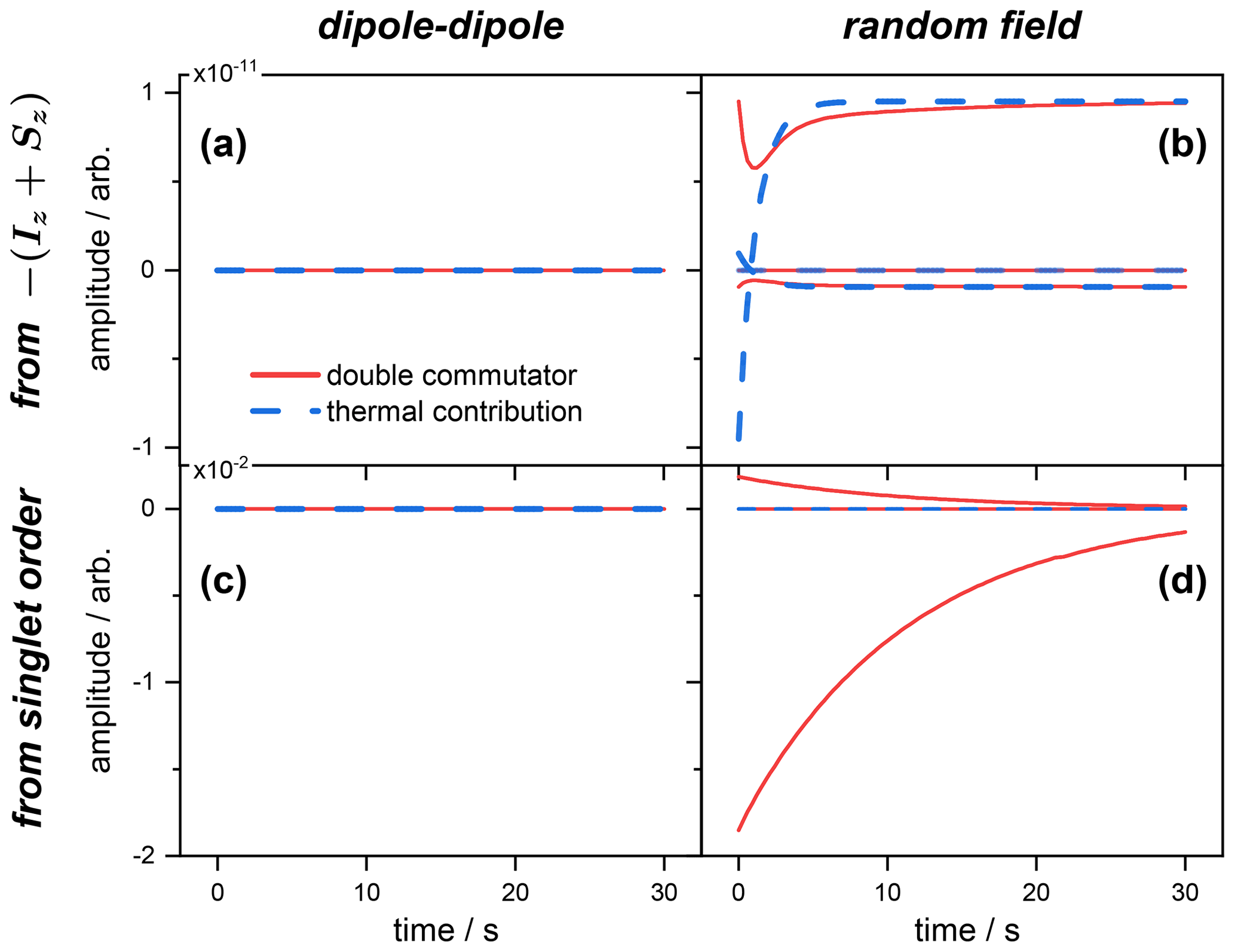
Contributions from both relaxation mechanisms to the expected values in Eq. (66) were computed for the spins prepared either in a singlet state or inverted from thermal equilibrium. The individual terms entering the first and second sums on the right-hand side of Eq. (66) are depicted for the case of the magnetization (Fig. 1) and singlet state (Fig. 2) operators. The time evolutions of all the contributions to the rate of change of the expected value of the operator 𝒪(t) are depicted. When the spins are initially prepared in the state , the thermal contribution (blue curve) to the rate of change of the magnetization has no effect, and the only contribution to comes from the double commutator (red curve). This is the case for both relaxation mechanisms, i.e., dipolar and random field fluctuations (Fig. 1a and b). Moreover, the values chosen for the simulation imply that the dipolar contribution (of the double commutator in this case) to the total relaxation rate is much larger than the one of the random field.
The situation is strikingly different when the spins are initially prepared in a singlet order. Here, the thermal correction (blue) is negligible with respect to the double commutator (red) contribution to the rate of change for the dipole–dipole mechanism only (Fig. 1c). In contrast, for terms originating from the random field relaxation, both thermal and dipolar terms are of comparable orders of magnitude (Fig. 1c). These are the terms that cannot be neglected in an approximate solution of Eq. (66). Figure 1c also shows that the dipolar contribution to increases with time, which is consistent with the progressive depletion of the singlet order (immune to dipolar relaxation). And, for random relaxation, which mainly affects the singlet order in this example, Fig. 1d illustrates the fact that the weight of the thermal contribution decays with time, with the concomitant increase in the double commutator term, which is also due to the progressive depletion of the singlet order.
The situation depicted in Fig. 2 is different and shows the rate of change of the expected value 〈𝒪〉(t), where , for the same initial state conditions as above. In this case, the dipole–dipole simply does not contribute to , as expected from symmetry considerations. This is, of course, the case whatever the initial state (inverted magnetization; see Fig. 2a) or singlet order (Fig. 2c). This illustrates the known fact that singlet state is immune to dipolar relaxation for symmetry reasons.
Alternatively, when the spins are prepared in the state, both thermal and double commutators contribute, albeit a negligible amount, showing that the spins evolve mostly towards magnetization (compare the scales with Fig. 1b) and that only a negligible part is transferred to a singlet order.
Interestingly, Fig. 2d shows that there is no thermal contribution (blue) to the rate , and that, starting from a singlet order, its evolution can be predicted by discarding the thermal terms of Eq. (66) and, therefore, retaining the simple double commutator expression for the relaxation master equation.
5.2.2 Singlet–triplet conversion
The recent achievement of the Lindblad approach was the description of the magnetization relaxation of a two-spin system prepared in a singlet state (Bengs and Levitt, 2020). In that paper, detailed balance was enforced through the Schofield (1960) procedure, whereby spectral density functions are built from classical ones through the following transformation:
where Jcl(ω) refers to the classical spectral density function. Equation (69) is one among several that have been proposed to make classical spectral density functions asymmetric so as to obey the detailed balance condition (White et al., 1988; Egorov and Skinner, 1998; Egorov et al., 1999; Ramirez and López-Ciudad, 2004; Frommhold, 1993). In Bengs and Levitt (2020), J(ω) was assumed to be any kind of spectral density function obtained through classical models, such as diffusion jumps, etc. The distinction between the left and right spectral densities that appear in the course of the conventional perturbative derivation of the master equation was not made there. Moreover, the detailed balance condition appears as an additional requirement, as this condition is not implied by Lindblad's approach that merely provides the general mathematical structure of the evolution equation obeyed by the density operator that complies with the requirements of quantum mechanics in the presence of a Markovian dissipative process (Lindblad, 1976; Alicki and Lendi, 2007).
In the following, we derive the evolution of the magnetization of a two-spin system, using the singlet–triplet population basis, and compare the results obtained by both approaches. As above (and in Bengs and Levitt, 2020) the relaxation super-operator is the sum of contributions from mutual dipole–dipole relaxation () and the interaction with a partially correlated random field (), as follows:
The irreducible tensor operator Tλμ representation is better suited to deriving analytical solutions for the problem at hand, where is expressed, according to Eq. (61), as follows:
The Tλμ are eigenoperators of the main Zeeman–Hamiltonian, and their expressions are shown in Appendix C. is the root mean square fluctuation of the random field acting on spin Ii, and in the isotropic case considered here, it is identical for both nuclei, so that . The coefficient describes the degree of correlation of the random field fluctuations on the 1 and 2 nuclei. By definition, . In order to simplify the notations, we will henceforth drop the subscript (κ12→κ).
In the extreme narrowing regime, where ωτC, ran≪1, the spectral densities become frequency independent and J(ω)≈2τ. The dipole–dipole and random field contributions to the longitudinal relaxation rate constant are given by, according to Eq. (61), the following:
where . Equations (72)–(77) were obtained using the SpinDynamica software (Bengs and Levitt, 2018). It is interesting to note that, in this model, the relaxation rates do not depend on the temperature, which is in contrast to Bengs and Levitt (2020). This is not due to any approximation; rather, it arises from the fact that , which is explicit in Eq. (72). Similarly, the singlet order relaxation rate is given by the following:
which does not depend on the temperature. For sake of comparison with the results of Bengs and Levitt (2020), we use the singlet–triplet population basis, where the singlet and triplet states are defined as follows:
where |α〉 and |β〉 denote the Zeeman spin states of an isolated spin (one-half) nucleus with z projection of and . In this representation, the population block of relaxation super-operator Eq. (71) is given by Eq. (76).
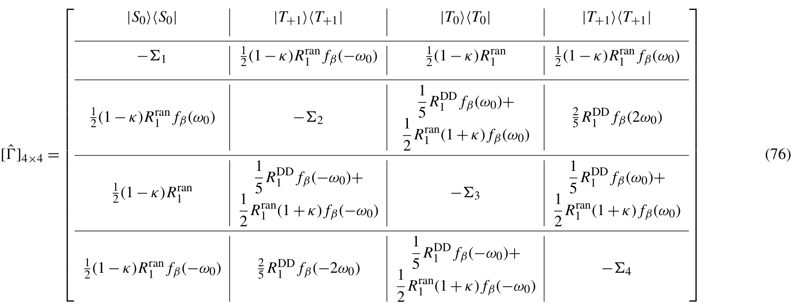
In Eq. (76), Σi denotes the sum of the terms alongside respective column. This matrix is very similar to one introduced in Bengs and Levitt (2020) but with the substitution of the term by fβ(ω).
In the high temperature limit, both terms become approximately equal, , and the difference between θ(ω) and fβ(ω) becomes significant only in the case of extremely low temperatures or very high frequencies. As could be expected in this limit, the time evolution of the z magnetization is given by the same bi-exponential behavior as in Bengs and Levitt (2020), as follows:
with the same coefficients and . The fact that A1 and AS are the ones found in Bengs and Levitt (2020) is expected because, in this limit, R1 and RS do not depend on the temperature factor. In the usual conditions of high but not infinite temperature, it is found that the next nonzero terms in the expansions of A1(β) and AS(β) are of the degree β2 and, therefore, do not contribute in the regime where ωβ≪1. These expressions can be found in Appendix D.
The foregoing discussion has shown that, in the high temperature approximation, the exact thermalization procedure of the spectral density function is irrelevant, as all models are equivalent in these conditions. Indeed, in a field of 23.5 T (1000 MHz resonance proton frequency), the temperature at which ℏωH≈kT, where both approaches may lead to significant differences, is T≈50 mK. These are unrealistic experimental conditions. Alternatively, the master equation of Eqs. (58)–(61) may well be of use in the context of dynamic nuclear polarization (DNP) to describe the electron spin–lattice relaxation outside of the high temperature limit through direct spin–phonon coupling at temperatures below 4 K and at high fields, where this process is predominant.
In the semi-classical viewpoint (as in Abragam, 1961, for instance), the effect of the bath is taken into account through a stochastic spin Hamiltonian, the spatial part of which is a function of the lattice variables and is a random function of time. It is usually understood that this approach does not comply with the Boltzmann equilibrium of the bath. Besides, the stationary state reached by the spin density operator is left undetermined by the master equation so that it must be enforced by the supplementary ad hoc assumption that the spins return to the Boltzmann distribution of the spin populations. A recent analysis by Bengs and Levitt (2020) showed that the usual semi-classical master equation was not able to predict the correct magnetization evolution of a two-spin system prepared in a singlet state.
Thus, the usual semi-classical inhomogeneous master equation provides erroneous predictions in this case. The latter is obtained when the thermal corrections to the double commutator part of the relaxation operator are retained to the first order in the largest eigenvalue , and the relaxation operator reduces to a double commutator (low-order case). However, the equilibrium density operator is not a stationary solution in this case, and therefore, a correction term is added to the master equation, leading to the same result as the usual semi-classical master equation (Hubbard, 1961). And so, when the low-order assumption is not verified, as in the case of a spin system prepared in the singlet state, this description becomes inconsistent.
As shown above, the non-commutation of the bath operators has critical consequences, leading to the lattice-temperature-dependent terms in the master equation, and it is only when the bath operators that one recovers the double commutator expression, with the additional property JL(ω)=JR(ω), so that the Kubo relation imposes an infinite lattice temperature. This illustrates how the finite temperature of the lattice is conveyed to the spins through non-commutation of the bath operators of the coupling Hamiltonian.
The conventional semi-classical approach, where spin–bath interactions are represented by random spin Hamiltonians, has the following two simultaneous consequences: the structure of the relaxation operator is affected in such a way that the master equation takes the form of a double commutator, and since JL(ω)=JR(ω), the system cannot evolve to a thermodynamic equilibrium associated with a finite temperature. In this case, the detailed balance property is conserved but only in the special case of infinite lattice temperature. In fact, since the detailed balance is statistical by nature, it is per se compatible with a semi-classical approach. If, on the other hand, a detailed balance is taken into account in the semi-classical theory of NMR relaxation, so that and the general relations Eq. (48) or (50) obeyed by correlation functions are retained, then it is easy to show from the symmetry properties of the spectral density function that the semi-classical Redfield equation (Abragam, 1961) in the following:
is obeyed with this definition of J(ω). However, the expected equilibrium density operator is not a stationary state of Eq. (78) in this case, which illustrates the (also known) fact that this condition alone is insufficient to completely determine the transition probabilities of the bath in the absence of a dynamical model for the latter. On the other hand, it is possible to describe the dynamics of a classical system where microscopic irreversibility, i.e., detailed balance, is ensured. This is straightforward from the definition of the correlation function of a phase variable in classical mechanics, , where L is the classical Liouvillian acting on the phase space (Evans and Moriss, 2008). In addition, general procedures have been used that provide Fokker–Planck or master equations for diffusion that obey the detailed balance condition, yielding classical spectral density functions that comply with the Boltzmann equilibrium distribution and the classical laws of motion of the bath (see, for instance, VanKampen, 1981; Risken, 1972; Wassam et al., 1980), in particular in the context of magnetic resonance (Stillman and Freed, 1980). As stated in several instances in this work, in the fully quantum approach, detailed balance is ensured by assuming that the bath is in a stationary state defined by a Boltzmann distribution of its energy states. Thus, the irreducible difference between the semi-classical and the fully quantized theory lies in the fact that the bath operators do not mutually commute, which prevents the expression in Eq. (26) from reducing to the double commutator. Both thermodynamic and quantum mechanical effects are thus entangled in the fully quantum mechanical treatment of relaxation.
In this derivation, the invariance of the trace to the circular permutations has been used, together with the fact that , since the bath is in a stationary state.
In the case of a homonuclear spin pair, the main Hamiltonian is defined as follows:
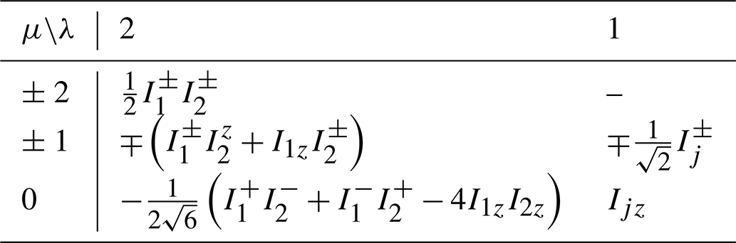
where , γ is the magnetogyric ratio, and B is the field strength. The eigenoperators for this Hamiltonian are summarized in Table C1. The eigenoperators are denoted by . The superscript (ij) indicates the angular momentum coupling of spins Ii and Ij, resulting in a spherical tensor operator of the total angular momentum λ and z-angular momentum μ.
Table C1Eigenoperators of Hamiltonian for a homonuclear coupled spin pair.
The coefficients from the Eq. (77) are in fact temperature dependent, as follows:
where the coefficients A1 and AS were shown before in the main text, and the coefficients C1 and CS are defined as follows:
The codes used in the simulations can be found at https://gitlab.com/phagost/linblad_simulations (Rodin, 2022).
No data sets were used in this article.
DA designed the research. DA and BAR performed the theoretical derivations and simulations and wrote the paper.
The contact author has declared that neither they nor their co-author have any competing interests.
Publisher’s note: Copernicus Publications remains neutral with regard to jurisdictional claims in published maps and institutional affiliations.
This article is part of the special issue “Geoffrey Bodenhausen Festschrift”. It is not associated with a conference.
This paper is dedicated to Geoffrey Bodenhausen, on the occasion of his 70th birthday. Bogdan A. Rodin acknowledges a Vernadski scholarship from the French embassy in the Russian Federation.
This research has been supported by the Russian Foundation for Basic Research (grant no. 20-53-15004) and by a PRC (Projet de Recherche Collaborative) funding from the Centre National de la Recherche Scientifique.
This paper was edited by Jean-Nicolas Dumez and reviewed by Christian Bengs, Alberto Rosso, Malcolm Levitt, Ranajeet Ghose, and one anonymous referee.
Abragam, A.: Principles of Nuclear Magnetism, Clarendon Press, Oxford, ISBN 978-0198520146, 1961. a, b, c, d, e, f, g, h, i
Alicki, R. and Lendi, K.: Quantum Dynamical Semigroups and Applications, Lect. Notes Phys., 717, ISBN 978-3-642-08985-5, 2007. a, b, c
Barbara, T. M.: The Lindbladian form and the reincarnation of Felix Bloch's generalized theory of relaxation, Magn. Reson., 2, 689–698, https://doi.org/10.5194/mr-2-689-2021, 2021. a
Bengs, C. and Levitt, M. H.: SpinDynamica: Symbolic and numerical magnetic resonance in a Mathematica environment, Magn. Reson. Chem., 56, 374–414, https://doi.org/10.1002/mrc.4642, 2018. a
Bengs, C. and Levitt, M. H.: A master equation for spin systems far from equilibrium, J. Magn. Reson., 310, 106645, https://doi.org/10.1016/j.jmr.2019.106645, 2020. a, b, c, d, e, f, g, h, i, j, k
Bloch, F.: Dynamical Theory of Nuclear Induction. II, Phys. Rev., 102, 104–135, 1956. a, b, c
Bloch, F.: Generalized Theory of Relaxation, Phys. Rev., 105, 1206–1222, 1957. a, b
Bloembergen, N., Purcell, E. M., and Pound, R. V.: Relaxation Effects in Nuclear Magnetic Resonance Absorption, Phys. Rev., 73, 679–712, https://doi.org/10.1103/PhysRev.73.679, 1948. a
Egorov, S. and Skinner, J.: Semiclassical approximations to quantum time correlation functions, Chem. Phys. Lett., 293, 469–476, 1998. a
Egorov, S. A., Everitt, K. F., and Skinner, J. L.: Quantum Dynamics and Vibrational Relaxation, J. Phys. Chem. A, 103, 9494–9499, 1999. a
Evans, D. J. and Moriss, G.: Statistical Mechanics Of Nonequilibrium Liquids, 2nd edn., Cambridge University Press, ISBN 9781483260457, 2008. a, b, c
Frommhold, L.: Collision-induced absorption in gases, Cambridge monographs on atomic, molecular, and chemical physics, vol. 2, Cambridge University Press, Cambridge, ISBN 978-0521019675, 1993. a
Goldman, M.: Formal Theory of Spin-Lattice Relaxation, J. Magn. Reson., 149, 160–187, 2001. a
Hubbard, P. S.: Quantum-Mechanical and Semiclassical Forms of the Density Operator Theory of Relaxation, Rev. Mod. Phys., 33, 249–264, https://doi.org/10.1103/RevModPhys.33.249, 1961. a, b, c, d, e
Jeener, J.: Superoperators in Magnetic Resonance, Adv. Magn. Reson., 10, 1–51, 1982. a
Kubo, R.: Statistical-Mechanical Theory of Irreversible Processes. I. General Theory and Simple Applications to Magnetic and Conduction Problems, J. Phys. Soc. Jpn., 12, 570–586, https://doi.org/10.1143/JPSJ.12.570, 1957. a
Levitt, M. and Bari, L. D.: Steady state in magnetic resonance pulse experiments, Phys. Rev. Lett., 69, 3124–3127, 1992. a
Lindblad, G.: On the Generators of Quantum Dynamical Semigroups, Commun. Math. Phys., 48, 119–130, 1976. a, b, c
Maimbourg, T., Basko, D. M., Holzmann, M., and Rosso, A.: Bath-Induced Zeno Localization in Driven Many-Body Quantum Systems, Phys. Rev. Lett., 126, 120603, https://doi.org/10.1103/PhysRevLett.126.120603, 2021. a
Nathan, F. and Rudner, M. S.: Universal Lindblad equation for open quantum systems, Phys. Rev. B, 102, 115109, https://doi.org/10.1103/PhysRevB.102.115109, 2020. a
Ramirez, R. and López-Ciudad, T.: Quantum corrections to classical time-correlation functions: Hydrogen bonding and anharmonic floppy modes, J. Chem. Phys., 121, 3973–3983, 2004. a
Redfield, A. G.: On the theory of relaxation processes, IBM J. Res. & Dev., 1, 19–31, https://doi.org/10.1147/rd.11.0019, 1957. a, b, c, d, e, f
Redfield, A. G.: The Theory of Relaxation Processes, Adv. Magn. Reson., 1, 1–32, 1965. a, b, c
Risken, H.: Solutions of the Fokker-Planck equation in detailed balance, Zeit. Phys., 251, 231–243, 1972. a
Rodin, B.: lindblad_simulations, Gitlab [code], https://gitlab.com/phagost/linblad_simulations, last access: 1 February 2022. a
Schofield, P.: Space-time correlation function formalism for slow neutron scattering, Phys. Rev. Lett., 4, 239–240, 1960. a
Stillman, A. E. and Freed, J. H.: Stochastic modeling of generalized Fokker–Planck equations. I., J. Chem. Phys., 72, 550–566, 1980. a
VanKampen, N.: Stochastic Processes in Physics and Chemistry, 3rd edn., North-Holland, ISBN 978-0444529657, 1981. a, b
Wassam, W. A., Balderas-Lopez, J. A., and Torres-Vega, G.: Stationarity of time correlation functions for globally linear classical systems and its consequences, J. Math. Phys., 31, 2466–2479, https://doi.org/10.1063/1.528990, 1980. a
White, J., Velasco, S., Hernandez, A. C., and Luis, D.: On the quantum time autocorrelation function, Phys. Lett. A, 130, 237–239, 1988. a
- Abstract
- Introduction
- Theory of spin relaxation in a thermal bath: a short review
- The Redfield equation is equivalent to the Lindblad form of the relaxation equation
- A pseudo-classical version of the Redfield equation
- Simplifications in the high temperature approximation
- Conclusion: a remark on semi-classical theory
- Appendix A: Derivation of Eq. (19)
- Appendix B: Evaluation of the terms of Eq. (44)
- Appendix C: Eigenoperators for a homonuclear coupled spin pair
- Appendix D: Expansion coefficient for the magnetization evolution solution
- Code availability
- Data availability
- Author contributions
- Competing interests
- Disclaimer
- Special issue statement
- Acknowledgements
- Financial support
- Review statement
- References