Radiation damping strongly perturbs remote resonances in the presence of homonuclear mixing

In this work, it is experimentally shown that the weak oscillating magnetic field (known as the “radiation damping” field) caused by the inductive coupling between the transverse magnetization of nuclei and the radio frequency circuit perturbs remote resonances when homonuclear total correlation mixing is applied. Numerical simulations are used to rationalize this effect.

1 Introduction

The inductive coupling between precessing magnetization and a radio frequency (RF) circuit creates an RF field, which, in turn, affects the evolution of the magnetization and, hence, the appearance of nuclear magnetic resonance (NMR) spectra. The existence of this phenomenon was first hypothesized by Suryan (1949), and a more rigorous theoretical description was later provided by Bloembergen and Pound (1954). The latter work introduced the term “radiation damping” (RD), an expression which, as several authors have previously stated (Abragam, 1961; Vlassenbroek et al., 1995; Hoult and Bhakar, 1997; Krishnan and Murali, 2013), is rather misleading, with both radiation and damping being called into question. The expression “radiation feedback” has been suggested as an alternative; however, this term is often used to designate active feedback circuits to enhance (Szoke and Meiboom, 1959; Hobson and Kaiser, 1975) or eliminate (Louisjoseph et al., 1995; Broekaert and Jeener, 1995) the effects of radiation damping. Another option, in analogy with quantum back action, could be “induction back action”. In order to avoid confusion, the term RD will, nevertheless, be employed in this work. When no other RF fields are present, the RD field rotates the magnetization that is responsible for the induced RF field towards its equilibrium direction (Bloom, 1957), parallel to the main field, leaving the norm unchanged (if it is homogeneous in space). In liquid-state NMR, this effect is usually weak and only noticeable when the magnetization is strong, either for nuclei in molar concentrations with high gyromagnetic ratios (in particular, solvents containing hydrogen) or when the polarization is enhanced. It increases with higher quality factors Q. The RD field strongly affects the resonances with frequencies close to the one that is at its origin (Schlagnitweit et al., 2012) and remote resonances that are directly coupled by scalar or dipolar interactions (Miao et al., 1999) or undergo chemical exchange (Chen and Mao, 1997) with the nuclei that induce RD. Subtle effects on remote resonances (Sobol et al., 1998) can affect sensitive difference experiments. Homonuclear isotropic mixing sequences which have been designed for total correlation spectroscopy (TOCSY), however, are very efficient at removing the chemical shift differences from the effective Hamiltonian (Braunschweiler and Ernst, 1983; Bax and Davis, 1985). In this work, it will be shown that RD, in the presence of suitable mixing sequences, can heavily perturb spins over a wide range of resonance frequencies.

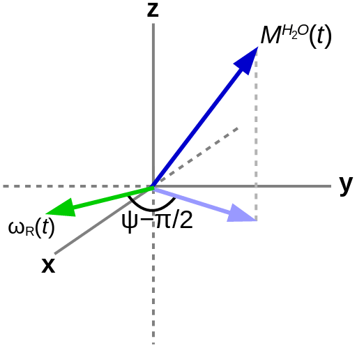
Figure 1 The RD field ω_R(t) (green arrow) lies in the xy plane. It has an amplitude that is proportional to the projection (light-blue arrow) of the water magnetization $M^{{\mathrm{H}}_{\mathrm{2}}\mathrm{O}}\left(t\right)$ (dark-blue arrow) onto the same plane and a phase of $\mathit{\psi }-\mathit{\pi }/\mathrm{2}$ with respect to this projection.

2 Materials and methods

All experiments have been performed on a Bruker NMR spectrometer in a field of 14.1 T (600 MHz proton frequency) equipped with a probe cooled by liquid nitrogen (“Prodigy”) with coils to generate pulsed field gradients along the z axis. This study has been done on a standard calibration sample that contained, among other substances, about 80 % H₂O and 20 % HDO (i.e., close to 100 M solvent protons) and 0.5 mM sodium 3-(trimethylsilyl)propane-1-sulfonate (DSS). At the experimental temperature of 298 K, the chemical shift difference between the solvent and the methyl protons is ca. 4.78 ppm (2868 Hz at 14.1 T, the water resonance being “downfield”, i.e., precessing at a higher negative frequency).

The variants of the selective TOCSY experiment (Davis and Bax, 1985; Kessler et al., 1986) used in this work, with an optional bipolar gradient pair for coherence pathway selection (Dalvit and Bovermann, 1995), are described in Fig. 2. A selective pulse applied to the solvent A, followed by a pulsed field gradient, can be inserted before the sequence so that the magnitude of the longitudinal magnetization $M_z^A$ can be controlled and, hence, the strength of the RD effect. If, for example, the pulse rotates the magnetization into the xy plane, RD should play no role in the remainder of the sequence, except if the dephased magnetization is (accidentally) refocused. If, instead of the transverse magnetization, one wishes to monitor the z component of the magnetization that remains after the homonuclear mixing sequence, a gradient followed by a $\mathit{\pi }/\mathrm{2}$ pulse can be inserted just before acquisition. For homonuclear transfer, an isotropic mixing pulse train, DIPSI-2 (Decoupling In the Presence of Scalar Interactions; Rucker and Shaka, 1989), has been chosen with an RF amplitude $\mathit{\gamma }{B}_{\mathrm{1}}/\mathrm{2}\mathit{\pi }=\mathrm{4.17}$ kHz (which corresponds to a duration of 60 µs for a $\mathit{\pi }/\mathrm{2}$ pulse). Selective excitation, either on the water or on the methyl protons, has been achieved with a Gaussian $\mathit{\pi }/\mathrm{2}$ pulse of 5 ms. The programs for the numerical simulation of the trajectories of the magnetization (see the Supplement for the code) and to extract the experimental peak intensities were written in the Python language. In particular, the evolution of the magnetization under the DIPSI-2 pulse train (governed by the set of nonlinear coupled differential Eqs. 1–3) was numerically evaluated with the SciPy integration libraries (Virtanen et al., 2020) using an explicit Runge–Kutta method of order 5 (RK5(4)) (Shampine, 1986).

3 Experimental results

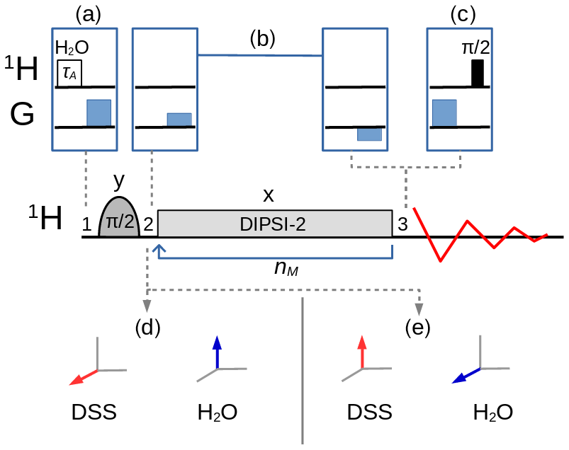
Figure 2 Selective TOCSY sequence. The magnetization of one nuclear spin species is rotated into the transverse plane by the selective $\mathit{\pi }/\mathrm{2}$ pulse, followed by a DIPSI-2 pulse train which is repeated n_M times. Neglecting relaxation and coherence transfer, the isotropic mixing DIPSI-2 sequence is designed to leave the magnetization unchanged (spin locked) across a wide band of frequencies centered on the RF carrier frequency. The selective pulse is cycled through (y, −y, −y, y) with a concomitant alternation of the receiver phase. (a) A selective pulse of duration τ_A applied to the water resonance followed by a pulsed field gradient can be inserted at position 1 to adjust the amplitude of the longitudinal components of the water magnetization between $+M_{\mathrm{eq}}^{\mathrm{A}}$ and $-M_{\mathrm{eq}}^{\mathrm{A}}$. (c) At position 3, a pulsed field gradient followed by a $\mathit{\pi }/\mathrm{2}$ pulse permits the detection of M_z. (b) An optional bipolar pulsed field gradient pair at positions 2 and 3 on each side of the mixing interval leads to a cleaner coherence pathway selection and a higher signal-to-noise ratio if the receiver gain can be increased, albeit at the cost of some signal decay due to translational diffusion (in addition, the gradient delays of about 3 ms cause a small loss due to transverse relaxation). In this work, the carrier frequency for all pulses was set either on the three methyl group resonances of DSS (leading to the situation – immediately after the selective $\mathit{\pi }/\mathrm{2}$ pulse – shown in d) or on the water resonance (shown in e).

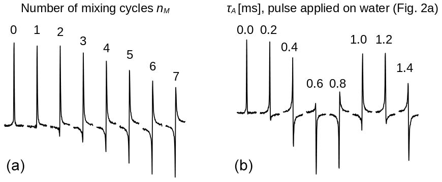
Figure 3 Spectra of the protons of the three methyl groups of DSS obtained with the experiment shown in Fig. 2 with the carrier set at the methyl resonance frequency (conditions before mixing as in Fig. 2d). The selective $\mathit{\pi }/\mathrm{2}$ pulse had a Gaussian profile of 5 ms. The strength of the RF amplitude during mixing was 4.17 kHz. (a) As the number of cycles n_M increases, the signal changes phase. Each pulse train cycle takes about 7 ms to complete. After 26 cycles, the resonance is back close to its initial phase (corresponding to a precession frequency close to 5.5 Hz). (b) The amount of z magnetization of H₂O is varied by applying a rectangular pulse with 250 Hz amplitude and a length τ_A (marked on top of each spectrum) to the water resonance followed by a pulsed field gradient (Fig. 2a) immediately before the sequence with n_M=26. All spectra have the same phase corrections.

First, the selective TOCSY experiment shown in Fig. 2 was applied with the RF carrier frequency set on the protons of the three methyl groups of DSS. The isotropic mixing module, DIPSI-2, consists of 36 RF pulses of constant amplitude and varying duration, applied along +x or −x, and is repeated n_M times (Rucker and Shaka, 1989). As the excited methyl spins S are not coupled, the mixing sequence acts as a spin lock and only a decay due to relaxation should be observed as n_M increases. Nevertheless, the spectra shown in Fig. 3a display a clear phase drift, making nearly a full turn at n_M=26. The change in phase depends strongly on the water $M_z^A$ magnetization at the beginning of the experiment, as can be seen from Fig. 3b: for n_M=26, immediately before the selective TOCSY sequence, an RF pulse applied to the H₂O resonance of varying length τ_A, followed by a gradient, has been inserted, so as to modify $M_z^A$ at will before the isotropic mixing sequence.

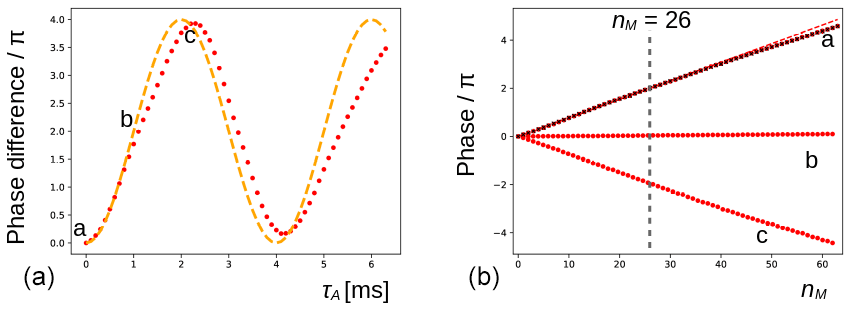
Figure 4 (a) The phase evolution of the methyl signal of DSS extracted from the experiment shown in Fig. 3b (n_M=26). The duration of the preparatory pulse applied on H₂O has been varied from 0 to 6.3 ms with increments of 0.1 ms (maximum nutation angle of ca. 3π). The orange dashed line shows the expected variation for an ideal RF pulse. (b) At positions a (0 ms), b (1.1 ms, no residual solvent magnetization), and c (2.2 ms, inversion), the phase evolution of the signal is shown (red dots) for $\mathrm{0}\le n_{\mathrm{M}}\le \mathrm{63}$ with increments of 1. The red dashed line corresponds to a linear fit of the first 32 points of a. The black crosses are recorded under the same conditions of a after inserting a bipolar gradient pair before and after the mixing period (as explained in Fig. 2) and are virtually undistinguishable from the red dots underneath.

In Fig. 4a, the phase variations of the latter experiment are plotted as a function of τ_A. Clearly, the magnitude of water magnetization that is present before the pulse sequence modulates the effect observed. The theoretical curve in orange predicts the evolution of the DSS resonance assuming that the phase is proportional to the initial longitudinal water magnetization, $M_z^A$, and the RF pulse on the water is ideal (i.e., with a nutation angle equal to ω₁τ_A). The deviations between the curve and the experimental points could be due to RF inhomogeneities, RD during the pulse applied to water, slight miscalibrations of the RF power, and a possible small misestimation of the initial phase shift. Moreover, as RD is a nonlinear phenomenon, it is not a priori clear that the theoretical curve should be followed. At positions a (τ_A=0 ms, when the water magnetization is unperturbed), b (τ_A=1.1 ms, when the water magnetization approximately vanishes), and c (τ_A=2.2 ms, when the water magnetization is approximately inverted), the phase evolution has been recorded as a function of number n_M of isotropic mixing cycles, as shown (red dots) in Fig. 4b. The dashed curve corresponds to a linear regression of the first half of the points of a, showing that the dephasing slows down slightly at a larger n_M (due to relaxation of the water magnetization). When a bipolar gradient pair is inserted to bracket the DIPSI-2 mixing sequence (black crosses), the effect of RD on the DSS resonance is almost undistinguishable from the same experiment that does not use gradients for coherence pathway selection.

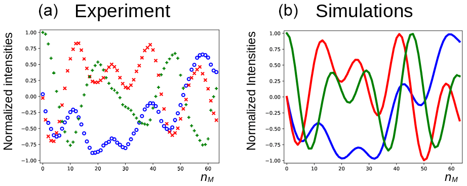
In Fig. 5a, the three components of the magnetization of the DSS methyl groups, recorded under the same conditions as Fig. 4 (curve a), are plotted as a function of n_M. Figure 6a shows the result of an experiment in which the carrier frequency has been moved to the solvent resonance and the amplitude of the selective Gaussian pulse has been increased in order to overcome RD effects during this pulse (so that the solvent magnetization is rotated into the xy plane). All other parameters were left unchanged. Here, the residual z component of the magnetization of DSS must be detected without changing the phase of the receiver for the different scans (the initial magnetization and the detected component have the same coherence order). Clearly, effects of the RD field are also observed in the latter experiment. Without RD, the magnetization is expected to stay along the z axis after each DIPSI-2 cycle. As in Fig. 5, the magnetization rotates away from its initial position, although its trajectory is much less regular.

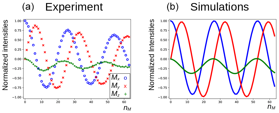
Figure 5 Evolution of the magnetization of the methyl resonance of DSS under the experimental conditions shown in Fig. 4 (curve a). For the calculations in panel (b), the RD rate and angle were set to $R_{\mathrm{R}}=\mathrm{33.4}\times \mathrm{2}\mathit{\pi }$ rad s⁻¹ and $\mathit{\psi }=\mathrm{30}{}^{\circ }$, respectively.

Figure 6 Same as Fig. 5 but with the carrier frequency set on H₂O (conditions before mixing as in Fig. 2e); the same symbols as in Fig. 5 correspond to the same components of the magnetization. The RD parameters for the simulations in panel (b) were the same as in Fig. 5.

4 Theory and discussion

In order to explain the experimental results, the homonuclear case of abundant spins A (H₂O), whose magnetization induces an RD field in the coil as shown in Fig. 1, and sparse spins S (the three methyl groups in DSS), whose RD interaction with the coil can be neglected, will be considered. In the rotating frame, the evolution of the two (uncoupled) types of spins can be described by the modified Bloch equations (Bloom, 1957):

$$\begin{array}{}\text{(1)}& {\displaystyle }\begin{array}{rl}{\displaystyle \frac{\mathrm{d}{M}_x^i\left(t\right)}{\mathrm{d}t}}& =-{\mathit{\omega }}_{\mathrm{0}}^i{M}_y^i\left(t\right)+{\mathit{\omega }}_{\mathrm{1}y}\left(t\right)M_z^i\left(t\right)-\mathit{\left\{}{c}_{\mathrm{R}x}\right(t)\\ & -s_{\mathrm{R}y}\left(t\right)\mathit{\left\}}{M}_z^i\right(t),\end{array}\text{(2)}& {\displaystyle }\begin{array}{rl}{\displaystyle \frac{\mathrm{d}{M}_y^i\left(t\right)}{\mathrm{d}t}}& ={\mathit{\omega }}_{\mathrm{0}}^i{M}_x^i\left(t\right)-{\mathit{\omega }}_{\mathrm{1}x}\left(t\right)M_z^i\left(t\right)-\mathit{\left\{}{c}_{\mathrm{R}y}\right(t)\\ & +s_{\mathrm{R}x}\left(t\right)\mathit{\left\}}{M}_z^i\right(t),\end{array}\text{(3)}& {\displaystyle }\begin{array}{rl}{\displaystyle \frac{\mathrm{d}{M}_z^i\left(t\right)}{\mathrm{d}t}}& =-{\mathit{\omega }}_{\mathrm{1}y}\left(t\right)M_x^i\left(t\right)+{\mathit{\omega }}_{\mathrm{1}x}\left(t\right)M_y^i\left(t\right)+\mathit{\left\{}{c}_{\mathrm{R}x}\right(t)\\ & -s_{\mathrm{R}y}\left(t\right)\mathit{\left\}}{M}_x^i\right(t)+\mathit{\{}{c}_{\mathrm{R}y}\left(t\right)+s_{\mathrm{R}x}\left(t\right)\mathit{\left\}}{M}_y^i\right(t).\end{array}\end{array}$$

Here, i is either spin A or S, ${\mathit{\omega }}_{\mathrm{0}}^i$ is the difference between the resonance frequency of spin i and the carrier frequency, ω_1x and ω_1y are the respective x and y components of the RF field during the mixing sequence, and the remaining terms in the equations are due to the RD field:

$$\begin{array}{}\text{(4)}& \begin{array}{r}{c}_{\mathrm{R}x}\left(t\right)={\mathit{\alpha }}_{\mathrm{R}}{M}_x^{\mathrm{A}}\left(t\right)\cos \left(\mathit{\psi }\right),s_{\mathrm{R}x}\left(t\right)={\mathit{\alpha }}_{\mathrm{R}}{M}_x^{\mathrm{A}}\left(t\right)\sin \left(\mathit{\psi }\right),\\ c_{\mathrm{R}y}\left(t\right)={\mathit{\alpha }}_{\mathrm{R}}{M}_y^{\mathrm{A}}\left(t\right)\cos \left(\mathit{\psi }\right),s_{\mathrm{R}y}\left(t\right)={\mathit{\alpha }}_{\mathrm{R}}{M}_y^{\mathrm{A}}\left(t\right)\sin \left(\mathit{\psi }\right),\end{array}\end{array}$$

where the amplitude of the RD field is ${\mathit{\omega }}_{\mathrm{R}}\left(t\right)={\mathit{\alpha }}_{\mathrm{R}}\sqrt{M_x^{\mathrm{A}}{\left(t\right)}^{\mathrm{2}}+M_y^{\mathrm{A}}{\left(t\right)}^{\mathrm{2}}}$, and its phase is determined by the angle ψ as indicated in Fig. 1. The proportionality constant α_R depends on the characteristics of the RF circuit:

$$\begin{array}{}\text{(5)}& {\mathit{\alpha }}_{\mathrm{R}}=\cos \left(\mathit{\psi }\right){\mathit{\mu }}_{\mathrm{0}}\mathit{\eta }\mathit{\gamma }Q/\mathrm{2},\end{array}$$

where μ₀ is the vacuum permeability, γ is the gyromagnetic ratio of the protons, η is the filling factor of the sample, and Q is the quality factor of the RF circuit. By a multiplication of α_R with the equilibrium magnetization of the abundant spins A, the use of the RD rate

$$\begin{array}{}\text{(6)}& R_{\mathrm{R}}={\mathit{\alpha }}_{\mathrm{R}}{M}_{\mathrm{eq}}^{\mathrm{A}}\end{array}$$

allows one to employ normalized magnetization vectors (i.e., divide all components of spin i by $M_{\mathrm{eq}}^i$) in Eqs. (1)–(4).

The evolution of the magnetization of both A and S nuclei during the DIPSI-2 pulse train has been numerically simulated using the above equations. First, the evolution of M^A(t) was determined. For spin S, Eqs. (1)–(3) reduce to the traditional Bloch equations, with the magnetization of spin A as a source of a time-dependent RF field. The values of the rate R_R and the angle ψ were estimated (the two values have independently been varied in the simulations) to give a qualitative agreement with the data, as shown in Fig. 5, rather than an exact fit. The combination of the two parameters is not unique, and a smaller angle ψ can be compensated by a larger value of R_R. The use of the RD parameters extracted from the signal of H₂O after a simple pulse-acquisition experiment does not lead to a good agreement. This is likely due to the fact that the RF circuit is not the same during signal acquisition as during the application of RF pulses (Marion and Desvaux, 2008; Pöschko et al., 2014). In Fig. 5, the agreement between simulations and experiments is quite satisfactory. The decay of the experimental curves is not only due to relaxation but also to RF inhomogeneities: the precession frequency of the DSS signal varies slightly with the RF amplitude, while the evolution of the z component is even more sensitive (see the Supplement). The perturbation is also present when the carrier during the mixing is set on a frequency different from DSS resonance. In the Supplement, simulations are presented for different offset frequencies.

For the curves in Fig. 6b, the same RD parameters as in Fig. 5 have been used. In the simulations, the fact that, due to RD effects, the water magnetization is not aligned along the x axis after the first $\mathit{\pi }/\mathrm{2}$ pulse has been taken into account (a phase shift of −18^∘ was determined experimentally). The agreement between experiments and simulations is adequate, considering the fact that neither RF inhomogeneity and calibration errors nor relaxation effects have been taken into account. Moreover, the evolution is very sensitive to the exact position of the water magnetization after the selective Gaussian pulse.

The deviation from quadrature between the RD field and the transverse magnetization of the solvent (ψ≠0) plays an important role. It can be particularly pronounced in cryogenically cooled probes (Shishmarev and Otting, 2011). Previous studies have shown the influence of this “non-ideality” on the evolution of the magnetization of the abundant spins. Sleator et al. (1987), Vlassenbroek et al. (1995), and Torchia (2009) demonstrated a polarization-dependent phase shift of the freely precessing signal, while Barjat et al. (1995) brought to light severe phase distortions in multiplets. Williamson et al. (2006) revealed that it causes asymmetries in Z spectra, potentially perturbing the observation of chemical exchange. It is instructive to investigate what happens with a far stronger RF amplitude, which much reduces possible imperfections in the DIPSI-2 sequence due to offset effects. In Fig. 7, several simulations of the trajectory of the DSS magnetization are presented with an amplitude of the RF field of the spin lock of 100.0 kHz. The carrier frequency was set on the water resonance, and the maximum mixing time was 0.200 s. Different initial conditions (shown above each graph) before the DIPSI-2 pulse train have been considered. When the initial magnetization of H₂O is aligned along one of the principal axes, the one of DSS nutates around this axis; when this is not the case (lower right corner), the trajectory of the DSS magnetization is more complex. When the initial solvent magnetization is put along the x axis, it stays continuously almost perfectly aligned along this axis and (neglecting relaxation) the RD field is constant, with one component parallel to the magnetization equal to ω_Rx=R_Rsin (ψ) and one term perpendicular to it along the y axis equal to ${\mathit{\omega }}_{\mathrm{R}y}=-R_{\mathrm{R}}\cos \left(\mathit{\psi }\right)$. The latter component is efficiently (in analogy to the offset term) averaged out from the effective Hamiltonian by the DIPSI-2 sequence, whereas the first component is unaffected because it commutes with the RF field at all times. Hence, the effect of the RD field on the dilute spins (after each completed DIPSI-2 cycle) is expected to be a nutation around the x axis with a frequency of $R_{\mathrm{R}}\sin \left(\mathit{\psi }\right)/\mathrm{2}\mathit{\pi }$. Indeed, this corresponds to the frequency of 16.7 Hz found in the graph on the top left corner. When the initial solvent magnetization is perpendicular (either along the z or the y axis) to the spin-lock field, the RD field becomes time dependent. The net effect is a nutation around the axis of the initial solvent magnetization with a frequency of about one-half compared with the previous one (in the Appendix, it is demonstrated that this is to be expected). When the initial magnetization of the solvent is oriented arbitrarily, the trajectory is less regular. The evolution of the solvent magnetization can also be strongly influenced by the much weaker RD field when the orientation of the initial magnetization is not along one of the three main axes (in the Supplement, the trajectories of the solvent magnetization under the same conditions as in Fig. 7 are shown).

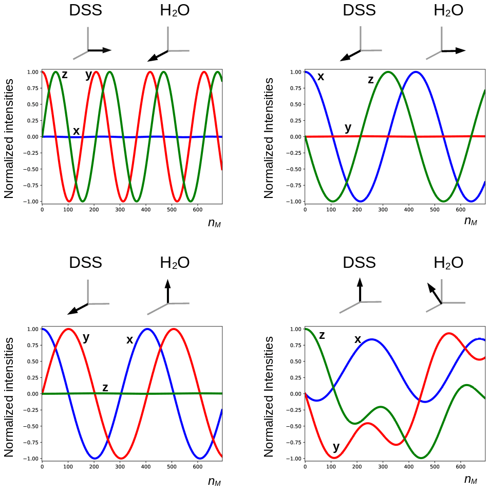
Figure 7 Simulated trajectories of the magnetization of the methyl groups of DSS under a DIPSI-2 pulse train with an RF amplitude of 100 kHz (90^∘ pulse of 2.5 µs), with the carrier frequency set on the water resonance. On top of each graph, the initial magnetization just before the spin lock is shown (in the lower right corner, $M_x^{\mathrm{A}}\left(\mathrm{0}\right)/M_{\mathrm{eq}}^{\mathrm{A}}=\mathrm{0.411}$, $M_y^{\mathrm{A}}\left(\mathrm{0}\right)/M_{\mathrm{eq}}^{\mathrm{A}}=-\mathrm{0.310}$, $M_z^{\mathrm{A}}\left(\mathrm{0}\right)/M_{\mathrm{eq}}^{\mathrm{A}}=\mathrm{0.857}$). The RD parameters used for the simulations and the color code of the curves are identical to those used in Figs. 5 and 6. For clarity, the curves are also labeled with the corresponding direction of the magnetization. The maximum number of cycles n_M = 694 corresponds to a duration of 0.200 s.

In the previous simulations, relaxation has not been taken into account. As it causes the magnetization of the solvent to diminish, its effect on the remote resonances should become weaker as the number of spin-lock cycles increases (as the regression line in Fig. 4 shows). In the Supplement, simulations with several different values of the transverse relaxation rates of the solvent $R_{\mathrm{2}}^{\mathrm{A}}$ illustrate this effect.

In this work, the selective TOCSY experiment has been investigated. For a (nonselective) two-dimensional TOCSY experiment, the situation is more complex, as, due to chemical shift evolution and RD, the orientations of the different magnetization vectors just before mixing depend on the duration of the indirect evolution period. In the Supplement, simulations are shown where the magnetization of both resonances is aligned along the x axis before the mixing period (much smaller effect) or where the magnetization of the water is aligned along the y axis while the one of DSS is along the x axis (effect comparable to Fig. 5).

The effect described in this article, which has been demonstrated using the DIPSI-2 mixing sequence, is expected to be present in other sequences which efficiently remove the chemical shift from the effective Hamiltonian. In the Supplement, simulations show that this is indeed the case for the MLEV-16 (Levitt et al., 1982) and the FLOPSY-16 (FLip-flOP SpectoscopY; Kadkhodaie et al., 1991) sequences. In contrast, a continuous wave spin lock with the same RF amplitude does not exhibit this effect.

The phenomenon shown in this work strongly depends on the characteristics of the probe. Similar results (not shown), albeit much smaller in magnitude, have been obtained at 18.8 T (800 MHz proton frequency) on a traditional “room temperature” probe.

5 Conclusions

It has been shown that, in the presence of sequences used for TOCSY mixing, RD can strongly perturb the evolution of the magnetization of spins that are neither directly coupled by scalar/dipolar interactions to the source spins nor have a nearby resonance frequency. As these types of mixing sequences efficiently remove the chemical shift differences from the effective Hamiltonian, the weak RD field affects resonances over a much wider range of frequencies than would be expected from its amplitude. Thus, counterintuitively, the RD field can cause the magnetization of remote resonances to precess notwithstanding the presence of a much stronger RF spin-locking pulse train. This effect increases with increasing RF amplitudes. Its magnitude depends on the instrumentation, the details of the pulse sequence, and the duration of the mixing time. It can be prevented by saturating or dephasing the magnetization of the spins that cause radiation damping before mixing.

Appendix A: Evolution of the passive spins under a strong DIPSI-2 field and a time-dependent RD field

The basic element of the DIPSI-2 sequence consists of nine pulses along the x axis of constant amplitude that alternate in sign with the following rotation angles ϕ_n for spins on resonance:

$$\begin{array}{}\text{(A1)}& \begin{array}{rl}R=& \mathrm{320}{}_x{\mathrm{410}}_{-x}{\mathrm{290}}_x{\mathrm{285}}_{-x}{\mathrm{30}}_x{\mathrm{245}}_{-x}{\mathrm{375}}_x\\ & {\mathrm{265}}_{-x}{\mathrm{370}}_x.\end{array}\end{array}$$

One full mixing cycle consists of a sequence

$$\begin{array}{}\text{(A2)}& R\overline{R}\overline{R}R,\end{array}$$

in which $\overline{R}$ denotes the same sequences of pulses, except for an opposite sign of the amplitude. The conditions of Fig. 7 are considered, i.e., the RF term of the Hamiltonian much larger than the other terms and the carrier frequency set on the resonance of the solvent. First, the situation in the top right corner of Fig. 7 will be looked at. The trajectory of the solvent magnetization is considered to be governed only by the dominant RF field, which means that it turns around the x axis and the RD field is entirely due to the y component of the solvent magnetization. Thus, for a spin I, during the kth pulse, the time-dependent Hamiltonian is given by

$$\begin{array}{}\text{(A3)}& \begin{array}{rl}{H}_{Ik}\left(t\right)& =\mathit{\left\{}{s}_k\right|{\mathit{\omega }}_{\mathrm{1}}|+R_{\mathrm{R}}\cos \left(\mathit{\psi }\right)\cos \left({\mathrm{\Phi }}_k+s_k\left|{\mathit{\omega }}_{\mathrm{1}}\right|t\right)\mathit{\}}{I}_x\\ & +R_{\mathrm{R}}\sin \left(\mathit{\psi }\right)\cos \left({\mathrm{\Phi }}_k+s_k\left|{\mathit{\omega }}_{\mathrm{1}}\right|t\right)I_y+{\mathit{\omega }}_{\mathrm{0}}^I{I}_z.\end{array}\end{array}$$

Here,

$$\begin{array}{}\text{(A4)}& {\mathrm{\Phi }}_k=\sum _{j=\mathrm{0}}^{k-\mathrm{1}}{s}_j{\mathit{\varphi }}_j,\end{array}$$

where s₀=1, s_n is the sign of the RF amplitude of the nth pulse, ϕ₀=0, ϕ_n is the absolute value of the rotation angle of the nth pulse, and t is the time starting from the beginning of the pulse. The offset term causes a negligible tilt of the RF field, is efficiently averaged out by one complete DIPSI-2 cycle, and can be omitted from further analysis. The time-dependent term that depends on I_x commutes with the RF Hamiltonian and averages out. It will also be omitted (this is not completely rigorous and can only be done if $\left|R_{\mathrm{R}}t\right|\ll \mathrm{1}$; hence, the higher the RF amplitude, the better the approximation). Consequently, Eq. (A3) becomes

$$\begin{array}{}\text{(A5)}& H_{Ik}\left(t\right)=a_k{I}_x+b\cos \left({\mathrm{\Phi }}_k+a_{k}t\right)I_y,\end{array}$$

where $a_k=s_k\left|{\mathit{\omega }}_{\mathrm{1}}\right|$, and b=R_Rsin (ψ). By going to a rotating (around the x axis) frame with an angular frequency of a_k, neglecting the counter rotating component, and tilting the frame by an angle Φ_k (also around the x axis), the Hamiltonian can be expressed as follows:

$$\begin{array}{}\text{(A6)}& H_{Ik}^{rt}\left(t\right)=b{I}_y/\mathrm{2}.\end{array}$$

The direction of the rotation depends on the sign of the RF amplitude. Thus, in its original frame, the propagator of the kth pulse is given by

$$\begin{array}{}\text{(A7)}& P_{Ik}=e^{-i{\mathrm{s}}_k{\mathit{\varphi }}_k{I}_x}{e}^{-i{\mathrm{\Phi }}_k{I}_x}{e}^{-i{\mathit{\tau }}_{k}b{I}_y/\mathrm{2}}{e}^{i{\mathrm{\Phi }}_k{I}_x},\end{array}$$

where ${\mathit{\tau }}_k={\mathit{\varphi }}_k/\left|{\mathit{\omega }}_{\mathrm{1}}\right|$ is the duration of the kth pulse. As ${\mathrm{\Phi }}_k+s_k{\mathit{\varphi }}_k={\mathrm{\Phi }}_{k+\mathrm{1}}$, the propagator of one full DIPSI-2 cycle (obtained by concatenating the propagators of all pulses) is

$$\begin{array}{}\text{(A8)}& \begin{array}{rl}{P}_{I\mathrm{D}}^y& =e^{-i{s}_K{\mathit{\varphi }}_K{I}_x}{e}^{-i{\mathrm{\Phi }}_K{I}_x}{e}^{-i{\mathit{\tau }}_{\mathrm{D}}b{I}_y/\mathrm{2}}{e}^{i{\mathrm{\Phi }}_{\mathrm{1}}{I}_x}\\ & =e^{-i{\mathit{\tau }}_{\mathrm{D}}b{I}_y/\mathrm{2}},\end{array}\end{array}$$

where K (=36) stands for the last index of the cycle, τ_D is the total duration of the cycle, and the latter equality is because ${\mathrm{\Phi }}_{\mathrm{1}}={\mathit{\varphi }}_{\mathrm{0}}=\mathrm{0}$ and ${\mathrm{\Phi }}_K+s_K{\mathit{\varphi }}_K=\mathrm{0}$ (ensured by Eq. A2). As this propagator leaves the initial solvent magnetization unchanged, it remains identical for subsequent cycles, and the effective Hamiltonian is equal to $R_{\mathrm{R}}\sin \left(\mathit{\psi }\right)I_y/\mathrm{2}$.

When the initial solvent magnetization is aligned along the z axis, the only difference is that the angle ${\mathit{\varphi }}_{\mathrm{0}}=\mathrm{90}{}^{\circ }$; hence, Eq. (A8) becomes

$$\begin{array}{}\text{(A9)}& P_{I\mathrm{D}}^z=e^{-i\mathit{\pi }{I}_x/\mathrm{2}}{e}^{-i{\mathit{\tau }}_{\mathrm{D}}b{I}_y/\mathrm{2}}{e}^{i\mathit{\pi }{I}_x/\mathrm{2}}=e^{-i{\mathit{\tau }}_{\mathrm{D}}b{I}_z/\mathrm{2}}.\end{array}$$

The nutation frequencies observed in Fig. 7 slightly deviate from the expected ones (about −2 % for the graph in the top right, and +2 % for the lower left corner). This is likely due to effects of the neglected counter rotating component, as this effect persists even when removing the offset and the RD term parallel to the RF field from the Hamiltonian in Eq. (A3). This component is rapidly modulated by the changes in sign of the RF amplitude between the pulses, so that it could affect a wider range of frequencies than can be expected from its amplitude. For other orientations (perpendicular to the RF field but not along either of the two principal axes) of the initial solvent magnetization, these perturbations do slightly modify the orientation of the solvent magnetization after each cycle, causing nonlinear effects and ever larger deviations with an increasing number of cycles.

When the carrier frequency is not set on the solvent resonance frequency, the analysis is more complex. In the Supplement, simulations similar to those in Fig. 5 are shown (carrier frequency set on the DSS resonance frequency) with varying RF amplitudes.