the Creative Commons Attribution 4.0 License.
the Creative Commons Attribution 4.0 License.
 | 15 Aug 2023
Performance of the cross-polarization experiment in conditions of radiofrequency field inhomogeneity and slow to ultrafast magic angle spinning (MAS)
Andrej Šmelko
Jan Blahut
Zdeněk Tošner
In this paper, we provide an analytical description of the performance of the cross-polarization (CP) experiment, including linear ramps and adiabatic tangential sweeps, using effective Hamiltonians and simple rotations in 3D space. It is shown that radiofrequency field inhomogeneity induces a reduction in the transfer efficiency at increasing magic angle spinning (MAS) frequencies for both the ramp and the adiabatic CP experiments. The effect depends on the ratio of the dipolar coupling constant and the sample rotation frequency. In particular, our simulations show that for small dipolar couplings (1 kHz) and ultrafast MAS (above 100 kHz) the transfer efficiency is below 40 % when extended contact times up to 20 ms are used and relaxation losses are ignored. New recoupling and magnetization transfer techniques that are designed explicitly to account for inhomogeneous radiofrequency fields are needed.
- Article
(5872 KB) - Full-text XML
- BibTeX
- EndNote


Cross-polarization (CP) is a remarkable experiment with a very long history (Schaefer, 2007). Hartmann and Hahn (1962) presented the theory of magnetization transfer in a two-spin system under conditions of double radiofrequency (RF) irradiation of a static sample. Pines et al. (1973) published their seminal work on proton-enhanced solid-state NMR of dilute spins such as 13C and 15N. While magic angle spinning (MAS) was already introduced by Andrew et al. (1958) and independently by Lowe (1959), it was only in 1977 that cross-polarization was successfully combined with sample rotation. The necessary modification of the Hartmann–Hahn conditions was described in Stejskal et al. (1977). After that, many modifications with variable amplitude irradiations on one or both RF channels were developed. Among them, simple linear ramps (Metz et al., 1994) and adiabatic sweeps (Hediger et al., 1995) became the most popular. Ramp CP was originally introduced to broaden the Hartmann–Hahn (HH) matching condition and to obtain uniform signal amplitudes. In the original publication, low MAS frequencies (below ∼ 10 kHz) were used, and the sweep could cover several HH conditions. At the same time, it was realized that the largest enhancement in signal intensity is obtained when the sweep covers only one HH condition (Metz et al., 1994). The RF amplitude sweep implies a partially adiabatic inversion of the spins and compensates for RF field inhomogeneities (Peersen et al., 1994; Hediger et al., 1995).
Until now, cross-polarization remains the main pulse sequence building block for magnetization transfers. At very high MAS frequencies, it becomes difficult to achieve HH zero-quantum matching where the difference between the two applied RF amplitudes is equal to the MAS frequency. Instead, the HH double-quantum matching condition must be used, in which the sum of the RF amplitudes equals the MAS frequency. The spin dynamics remain the same with the exception that negative intensities are obtained (Meier, 1992). Cross-polarization is thus applied over an exceptionally wide range of conditions: from experiments using static samples to MAS experiments with rotation frequencies above 100 kHz.
The most widespread coil design used by all vendors in most of the MAS solid-state NMR probes is a solenoid. Its simple design, large filling factor, high conversion ratio from RF power to RF field and its possibility of being integrated into circuits tuned to multiple frequencies are among the major benefits. The main drawback is its inhomogeneous RF field, which quickly decays towards the end of the coil, where the RF amplitude is reduced to about 50 % of the value achieved in the coil center. Several other strategies have been proposed to design NMR coils that are compatible with MAS and provide improved RF field homogeneity. Variable pitch coils were proposed by Idziak and Haeberlen (1982) and recently explored by Martin and coworkers, who proposed 3D-printed templates for easy manufacturing (Kelz et al., 2019). An interesting alternative was proposed by Privalov et al. (1996) using variable ribbon-width coils that improve RF homogeneity not only along the coil axis but also in the radial direction. Another type of coil was designed for so-called E-free probes, which minimize sample heating effects induced by high-power RF irradiation. These coils also show improved RF field homogeneity (Krahn et al., 2008). All strategies have benefits and disadvantages. Variable-pitch coils provide a lower RF conversion ratio and thus lower sensitivity. E-free probes consist of separated coils for the high- and low-frequency RF channels, which potentially leads to different RF field profiles and imbalances between these channels. Worth mentioning is the recent cryo-CP-MAS probe technology that is reported to provide excellent RF field homogeneity (Hassan et al., 2020).
RF field inhomogeneity is a concern for the performance of virtually all NMR experiments. Specifically, it affects the sensitivity of the cross-polarization experiment, since the Hartmann–Hahn matching is violated at different positions within the sample as a consequence of the modulation of the RF amplitudes due to inhomogeneity. An experimental example of this volume-selective behavior of the cross-polarization experiment is presented in the work of Tošner et al. (2018). In biomolecular applications, it is difficult to prepare large quantities of isotopically labeled samples, and only limited amounts of material are available that do not allow us to completely fill the MAS rotor. To yield the highest possible sensitivity, samples are typically packed around the center of the coil, and the problem of RF field distribution is reduced. However, the rotors for ultrafast MAS are small and can be completely filled with sample. Under these conditions, RF inhomogeneity comes up as a concern in its full range. With faster MAS and correspondingly smaller rotors that contain less material, we again face sensitivity issues. It is obviously desirable that the whole sample contributes to the NMR signal. At this point, it appears that the inhomogeneity of the RF field is the prevailing challenge for the development of new solid-state NMR methods.
In this tutorial article, we summarize the principles of the cross-polarization (CP) experiment and focus on the effect of RF field inhomogeneity. For demonstration purposes we limit our treatment to an isolated heteronuclear pair of spin- nuclei that are coupled via the dipole–dipole interaction. We assume that there is no chemical shift interaction. Using average Hamiltonian theory and simple 3D rotations we explain the process of magnetization transfer assuming different amplitude-swept CP variants. We show that the total signal measured after the CP transfer decreases with increasing MAS frequency. The effect is amplified for small dipolar couplings. We numerically optimize linear ramp and adiabatic tangential sweep experiments to identify the conditions for the best performance as a function of the dipolar coupling constant, contact time and MAS frequency. Neither of these techniques under any condition fully compensates for RF field inhomogeneities. The most striking example of low efficiency is the CP transfer between a 15N nucleus directly bonded to a 13C atom involving a dipolar coupling constant of about 1 kHz. With the forthcoming MAS technology in mind that can reach MAS frequencies of up to 200 kHz, we predict that only 20 % of the sample will contribute to the NMR signal after a CP mixing time of 10 ms. It clearly calls for the development of alternative magnetization transfer techniques that are suitable for ultrafast MAS NMR experiments.
A theoretical description of the cross-polarization phenomenon can be found in many solid-state NMR textbooks. Here, we revisit the relevant parts and focus on visualization of the magnetization transfer process during variable-amplitude sequences, following the description presented by Rovnyak (2008). In the following, we assume an isolated spin pair. A more general description that considers the surrounding spins and homonuclear interactions within an INS spin system can be found, for example, in the work of Vega and coworkers (Marks and Vega, 1996; Ray et al., 1998). This issue has been reviewed in the context of ultrafast MAS by Emsley and coworkers (Laage et al., 2009), concluding that the perturbation effects of homonuclear interactions diminish with increasing spinning rate. The authors infer that the behavior of the CP experiment at very fast spinning in a INS spin system is reminiscent of a 13C–15N spin pair, which we would like to analyze in the following in detail.
2.1 Hamiltonian decomposition into zero-quantum (ZQ) and double-quantum (DQ) subspaces
We start with the Hamiltonian that contains the dipole–dipole interaction and the radiofrequency fields with amplitudes ωI and ωS applied on resonance to spins I and S, respectively.
The dipolar term is time dependent due to magic angle spinning (angular frequency ωR) and can be expressed as
where bIS is the dipolar coupling constant () in units of hertz and β and γ are the Euler angles relating the orientation of the dipolar vector rIS to the rotor axis (the α angle is irrelevant as the dipolar coupling tensor has a vanishing asymmetry).
Subsequently, the reference frame is transformed into the tilted frame where the radiofrequency fields are linear with Iz and Sz, while the dipolar term becomes transversal. This transformation is represented by a rotation around (Iy+Sy) and we obtain
Table 1Fictitious spin- operators in zero-quantum and double-quantum subspaces.
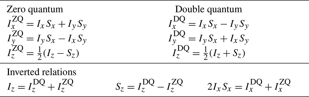
This form of the Hamiltonian allows decomposition of the spin dynamics problem into two separate subspaces, the zero-quantum (ZQ) and the double-quantum (DQ) subspace. The ZQ and DQ subspaces can be represented using fictitious spin- operators that are defined in Table 1.
The Hamiltonian can then be written as
2.2 Magnetization transfer in the static CP experiment
The magnetization transfer process in the tilted frame is described by a transition from Iz into Sz. The action of RF pulses and the dipolar interaction on the spin state Iz in the tilted frame are evaluated independently in the ZQ and DQ subspace, working with the initial spin states and , respectively. If the sample is static, the zero-quantum Hartmann–Hahn condition is and the Hamiltonian in Eq. (7) reduces to (dIS is time independent). The spin state represented by the operator is rotated around the axis as a consequence of the dipolar interaction. Simultaneously, the spin state evolves in the DQ subspace. We can assume that ωI+ωS is much larger than dIS. The effective rotation axis is thus oriented along ; see Eq. (8). As a result, HDQ has no effect on the state. This is summarized in the following equations.
The Iz spin state is transformed into Sz when , resulting in a full inversion of the operator.
For the double-quantum Hartmann–Hahn condition , the rotation occurs in the DQ subspace. By analogy with the previous case, we assume . Under this precondition, the ZQ spin state is not changed.
For , the operator is inverted resulting in the generation of the operator −Sz. Note that the double-quantum Hartmann–Hahn condition yields negative signal intensity.
The dipolar coupling is an orientation-dependent interaction. To yield the magnetization transfer dynamics for a powder sample, the ensemble of all possible crystallite orientations has to be accounted for. The powder-averaged inversion efficiency is lower since the condition of a complete transfer, , will hold only for a single orientation.
2.3 Magic angle spinning and average Hamiltonians
In the case of MAS, the Hamiltonians become time dependent. The analysis is then performed using average Hamiltonian theory (AHT) employing the Magnus expansion. A tutorial on AHT principles was presented by Brinkmann (2016). To retain fast convergence of the Magnus series, the Hamiltonian is expressed in an appropriate interaction frame. Equation (2) implies four resonance conditions upon transformation into a new rotating frame in which the periodic modulations of dIS(t) are removed by application of RF fields. These resonance conditions are associated with the characteristic frequencies nωR with . We choose and focus on the ZQ subspace. In general, transformation to a new reference frame is described using a propagator UT(t). This propagator transforms the Hamiltonian according to
In this case, . The transformation can be regarded as a rotation around with a frequency −ωR. The second term in Eq. (15) is a Coriolis term which introduces the term into the transformed Hamiltonian.
The first-order Hamiltonian is the time average over the modulation period
The integral over the time-dependent parts in Eq. (16) is evaluated as follows (making use of trigonometric identities):
We thus obtain the first-order average Hamiltonian in the ZQ subspace as
The Hartmann–Hahn condition is corrected to account for the rotation of the sample and has the form . In this case, the component of along the axis vanishes and the dipolar interaction results in a rotation around an axis in the transversal plane, with a phase depending on γ. For each crystallite, the spin state is flipped away from the z axis generating a transversal component. These transversal components are equally distributed with respect to the γ angle and average to 0 in a powder sample. Only the projection on the axis is relevant, and we can therefore arbitrarily set γ=0.
The calculation can be repeated for other choices of n and the following zero-quantum average Hamiltonians are obtained:
The fast convergence of the Magnus expansion is maintained and the proper description of spin dynamics by an average Hamiltonian is valid in the vicinity of the Hartmann–Hahn condition (. The RF amplitudes ωI and ωS may become time dependent if a linear ramp or an adiabatic sweep is applied. In any case, we assume that RF changes are slow compared to the MAS frequency to ensure the validity of this treatment.
The analysis is completed by inspecting the spin dynamics in the DQ subspace. We apply the same procedure as for the ZQ subspace, yielding
For the zero-quantum condition, it is assumed that the term dominates the average Hamiltonian ; i.e., for all . Under these conditions, the initial state remains unchanged. However, these conditions might be violated for large RF amplitude sweeps or in the case of substantial RF field inhomogeneity.
2.4 CP matching profiles
For constant RF amplitudes, the magnetization transfer process can be analytically described to derive the so-called CP matching profiles (sometimes dubbed Hartmann–Hahn fingers). This derivation was previously published in Levitt (1991) and Wu and Zilm (1993). It is assumed that both the ZQ and DQ Hartmann–Hahn conditions are independent. We reiterate the calculation for the matching condition and focus first on the ZQ Hamiltonian given in Eq. (19). We proceed with the final transformation into the effective field of the Hamiltonian. The Hamiltonian can be represented as a vector in the xz plane. This vector has an angle ϕ with the x axis. The transformation into the effective field is described by a rotation around by an angle −ϕ, which is equivalent to the application of the propagator . It makes the x axis of the new frame coincide with the effective Hamiltonian vector. Note that the Coriolis term in Eq. (15) is absent because UT is time independent. The effective Hamiltonian can be written as
The initial spin state transforms into in the effective field frame and evolves with a frequency around the effective field axis :
The result is transformed back from the effective field frame into the ZQ subspace as . This yields
Equation (25) describes the trajectory of the operator in the ZQ subspace under the influence of the RF pulses applied in the CP experiment. For evaluation of the magnetization transfer process, only the projection on the axis is important. We assume that there is no evolution in the DQ subspace; i.e., . The initial Iz operator thus evolves as (recall )
We obtain the CP transfer efficiency in the vicinity of the zero-quantum condition (n) by collecting the terms in front of the Sz operator:
A similar calculation for the double-quantum Hartmann–Hahn condition yields
Note the negative sign of the transferred magnetization for the double-quantum Hartmann–Hahn transfer. Equations (27) and (28) are identical to the result of an alternative derivation presented by Marica and Snider (2003). The CP MAS matching profile has the form of a Lorentzian function with a width that is dependent on the dipolar coupling bIS and the crystallite orientation (Euler angle β) that are included in the gn factors. In powders, a quantitative magnetization transfer is not possible as a consequence of the dependence of the size of the effective dipolar coupling on orientation. The magnetization transfer efficiency under MAS is independent of the γ angle. This property is referred to as γ encoding. The powder average is obtained by evaluation of the integral:
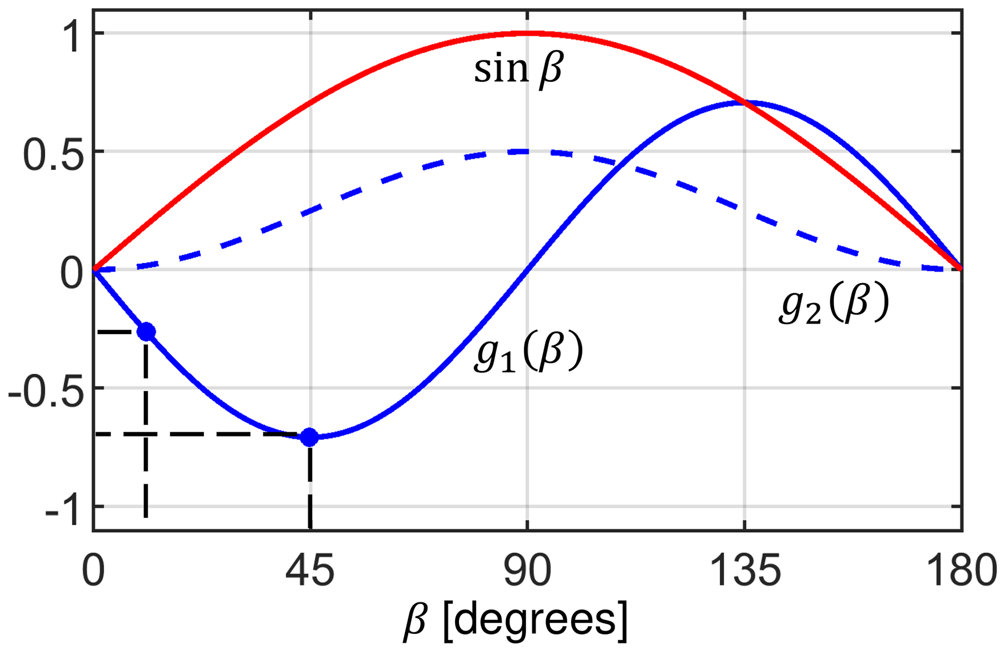
Figure 1Dipolar coupling scaling factors g1(β) (solid blue line) and g2(β) (dashed blue line) defined in Eqs. (3) and (4). The red curve represents the relative probability of finding a specific orientation in a powder sample. This weighting factor is employed for the calculation of the transfer efficiencies ϵ in Eq. (30). β angles with β = 15 and 45∘ are used for the visualization of the spin dynamics in the “Results and discussion” section.
2.5 Radiofrequency field inhomogeneity
Radiofrequency fields in MAS probes are realized using solenoid coils. However, a solenoid produces a rather inhomogeneous distribution of magnetic fields across the sample (Tošner et al., 2017). Moreover, as the sample rotates, individual spin packets travel along circles through a spatially inhomogeneous RF field which is determined by the helical geometry of the solenoid coil. This RF inhomogeneity introduces periodic modulations of both the RF amplitude and phase. For the special case of the CP experiment, it was recently shown that these temporal modulations have a negligible effect (Aebischer et al., 2021) and will be ignored in the present treatment. In addition, the distribution of the RF fields depends on the frequency (Engelke, 2002) and can be influenced by different balancing of the RF circuitry on different channels (Paulson et al., 2004). For simplicity, we assume the RF field distributions to be equal for the I and S spins and disregard the radial dependency. The effect of RF field inhomogeneity on the CP experiment was previously studied by Paulson et al. (2004) and Gupta et al. (2015). An example of the distribution of the RF field along the coil axis, denoted ξ(z), is shown in Fig. 2. As noted by Gupta et al. (2015), the profile deviates from a Gaussian function and is described well by a power law dependence. In our study, we use the B1 profile calculated according to Engelke (2002).
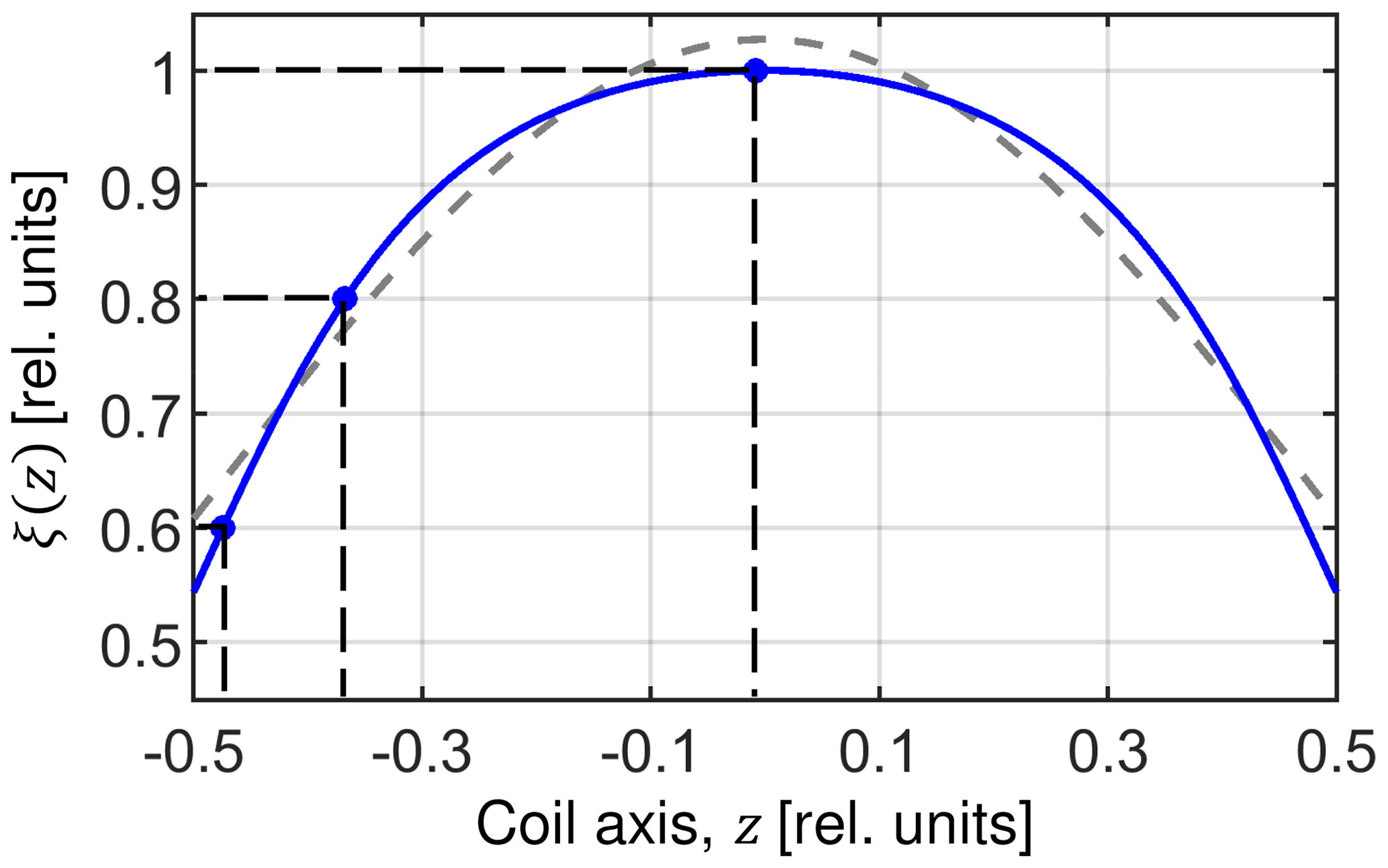
Figure 2RF field inhomogeneity profile along the axis of a solenoid coil. The profile is calculated according to Engelke (2002) assuming a coil length of 7.9 mm, a diameter of 3.95 mm and seven turns (blue line). The dashed gray line represents a fit of the RF profile assuming a Gaussian function suggested by Paulson et al. (2004). The power law relation introduced by Gupta et al. (2015) yields a perfect fit of the theoretical behavior and exactly matches the blue curve. Values ξ = 0.6, 0.8 and 1.0 are used in the “Results and discussion” section to visualize spin dynamics.
The distribution of RF field amplitudes enters the formulas of the CP experiment using the substitution
where and refer to the nominal RF amplitudes realized in the center of the coil (z=0 where ξ(0)=1). The overall experimental efficiency corresponds to the integral over the sample volume weighted by the detection sensitivity of the coil. According to the reciprocity theorem (Hoult, 2000), the sensitivity is proportional to the RF field. We assume that the sample extends over a length l and is placed symmetrically within the solenoid coil.
The normalization factor w is given as
It is not possible to match the Hartmann–Hahn conditions for the whole sample volume. Assuming that the zero-quantum condition is fulfilled for the nominal RF amplitudes, i.e., , we get
and
Equation (34) shows that in the case of an inhomogeneous RF field, the prevailing component along the operator in the effective Hamiltonian is proportional to the MAS frequency ωR, multiplied by the order of the recoupling condition n. The effect of RF amplitude mismatch on spin dynamics is more pronounced for small dipolar couplings, bIS, which is reflected in the width of the CP MAS matching profiles derived above. Thus, we could analytically derive a dependence of the performance of the CP experiment on the MAS frequency.
2.6 Linear ramp and adiabatic sweep
The most popular way to overcome the limitations of the constant amplitude CP and the RF mismatch at different positions of the sample is the use of a linear ramp or an adiabatic tangential sweep on one of the RF channels. We can define
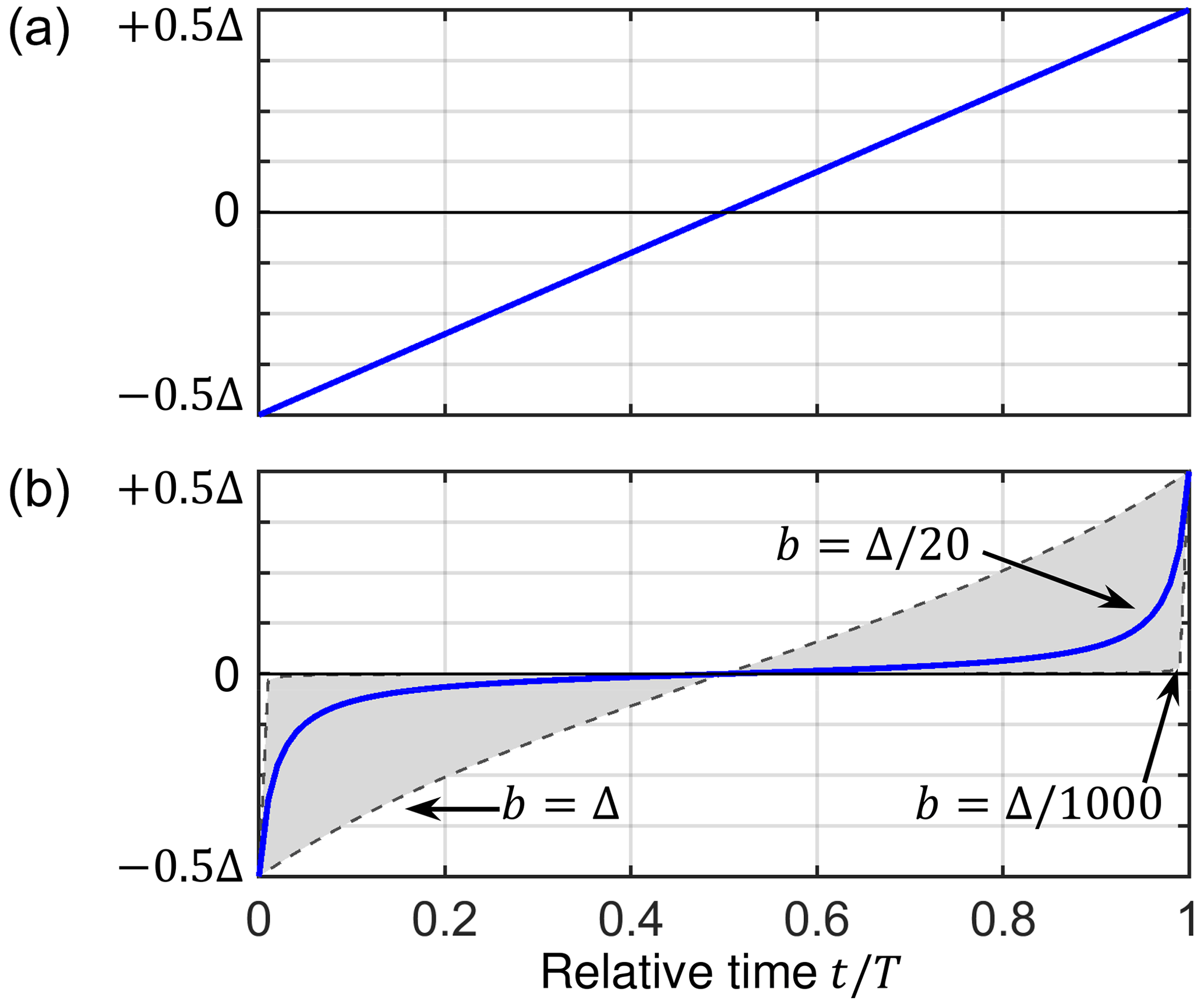
where the function f(t) describes the sweep from to over time . The function f(t) can be defined for the linear ramp as
and for a tangential sweep as
where b parameterizes the curvature of the sweep. Values for b are typically in the range of . For , f(t) is almost constant except for the end points where the function changes rapidly. For b=Δ, f(t) approaches the linear ramp. The influence of b on the shape is illustrated in Fig. 3. During a truly adiabatic transfer, the effective field is aligned with the initial magnetization along the axis and changes its orientation slowly towards . The spin state is locked along the effective field and is inverted as well (Hediger et al., 1995). The adiabaticity condition is given as
where ωeff is defined in Eq. (22) and the angle ϕ is given in Eq. (23). Adiabatic inversion pulses have been an integral part of the NMR toolbox for a long time (Baum et al., 1985). There is, however, a substantial difference between broadband inversion pulses and cross-polarization. Inversion pulses allow us to manipulate the effective field along z and x directions, corresponding to offset and RF amplitude, respectively. In the CP experiment, the x axis component of the effective Hamiltonian is fixed and is determined by the dipolar coupling; see Eqs. (19) and (20). In addition, perfect alignment of the effective field with the initial state is difficult to achieve as the RF amplitudes are restricted to the vicinity of the Hartmann–Hahn condition.
2.7 RF amplitude sweeps and RF field inhomogeneity
In the following, we aim to include RF field inhomogeneity in the description of the RF amplitude sweep of Eq. (35). We assume that the zero-quantum Hartmann–Hahn matching conditions are fulfilled in the middle of the sweep and in the center of the coil for the nominal RF field amplitudes, i.e., for . The component of the Hamiltonian then becomes
and
Now, the sweep function f(t) is scaled by the RF field inhomogeneity factor ξ(z). At the same time, the center of the sweep is shifted by an amount proportional to the MAS frequency ωR. In Fig. 4, the sweep range is depicted in green as a function of position along the coil axis. Spins located in volume elements towards the ends of the coil where the RF field is smaller experience RF amplitude sweeps that do not cover the recoupling condition at all (e.g., for ξ = 0.8 in Fig. 4a). This is another example of how increased MAS frequencies impact the cross-polarization experiment and cause a decrease in performance.
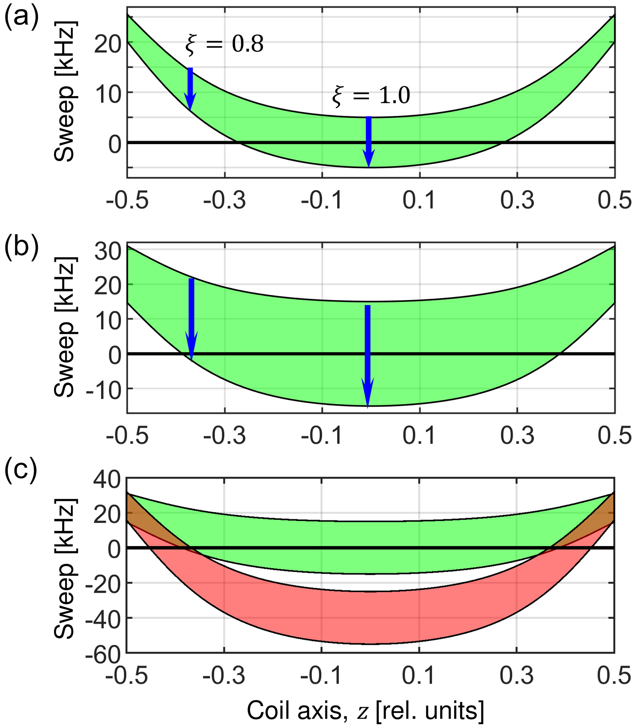
Figure 4Visualization of the RF sweep ranges as a function of the position of a particular spin packet along the coil axis. The Hartmann–Hahn resonance condition is artificially defined for a sweep frequency 0 kHz. (a) The sweep range (green area) is evaluated according to Eq. (39) for and assuming a MAS frequency of 50 kHz. The blue arrows indicate the direction of the sweep for an RF inhomogeneity factor of ξ = 0.8 and 1.0. The sweep amplitude Δ corresponds to 10 and 30 kHz in (a) and (b), respectively. (c) Overlay of the RF amplitude sweeps evaluated for the ZQ () matching condition (Eq. 39, green) and DQ () matching condition (Eq. 41, red) with nominal RF amplitudes = 95 kHz and = 45 kHz. These values were selected to demonstrate that the ZQ matching condition is satisfied in the center of the coil, and simultaneously a DQ is encountered for spin packets in regions of the sample where the RF amplitudes are scaled down by the RF field inhomogeneity.
When setting the numerical values of RF amplitudes , and the sweep range Δ, it can happen that double-quantum conditions are fulfilled in some places within the sample when the values are scaled by the RF field inhomogeneity. The double-quantum conditions are governed by the formula
which is represented in red in Fig. 4c. While the values and do satisfy the zero-quantum condition around the center of the coil, at the same time, they satisfy the double-quantum condition towards the ends of the coil (places where the red area crosses the zero value). As a result, there are parts of the sample that produce a positive magnetization transfer and parts that experience a negative transfer. Thus, the overall efficiency of the experiment is decreased.
3.1 CP matching profile
Experimentally, optimal cross-polarization conditions are found in experiments in which the RF amplitude on one of the RF channels is systematically varied to yield the highest sensitivity. If the Hartmann–Hahn recoupling condition is very narrow, this can be difficult as many repetitions with a small increment in the RF amplitude are required. In the Theory section, we derived analytical formulas for the CP matching profiles for constant RF amplitudes. We have found that for a homogeneous RF field distribution, the width at half height of the recoupling condition is governed by the size of the dipolar coupling and can be estimated as 0.468bIS after powder averaging. Both the width and the maximal transfer efficiency are independent of the MAS frequency. A maximum transfer of 73 % is achieved for mixing times satisfying the condition tbIS=1.7 for the n = ± 1 recoupling conditions. The same efficiency is obtained for the n = ± 2 conditions. However, due to the different spatial dependence and scaling factors in g1 and g2 terms (Eqs. 3 and 4), the maximum is achieved there for mixing times tbIS=2.4. These facts are well known and are presented graphically in Fig. 5. Figure 5a shows the CP matching profile calculated using Eqs. (27) and (30) for and assuming a dipolar coupling constant bIS of 1, 10 and 20 kHz, which are the characteristic values for 13C–15N, 1H–15N and 1H–13C spin pairs, respectively. 〈ϵZQ,1〉powder is represented as a function of the RF amplitude mismatch with respect to the exact Hartmann–Hahn.
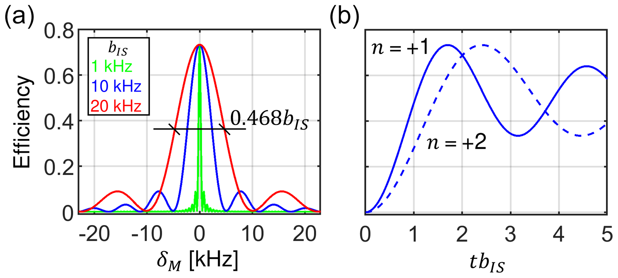
Figure 5Properties of the constant amplitude CP experiment assuming homogeneous RF fields. (a) The width of the CP matching profile around the zero-quantum () Hartmann–Hahn matching condition depends on the dipolar coupling strength bIS. (b) Magnetization buildup of the transferred magnetization for the and matching condition. Independently of the MAS frequency and bIS, the condition reaches the same maximum, however, at longer mixing times. The curves were calculated using Eqs. (27) and (30).
For inhomogeneous RF fields, the CP matching profile can be quantitatively described by inserting Eq. (31) into Eq. (27) and taking the average in Eq. (32). Figure 6a shows the influence of inhomogeneous RF fields and the induced asymmetric broadening of the matching profile . Clearly, the maximal transfer efficiency substantially decreases with increasing MAS frequency.
A closer inspection of the CP matching profiles in Fig. 6a reveals that the maximum overall transfer efficiency is not reached for the exact ZQ () condition with , corresponding to δM = 0. In practice, it is advantageous to set a little higher and thus shift the volume element where the Hartmann–Hahn condition is matched away from the center of the coil. This allows us to partially compensate for the destructive effect of the RF field inhomogeneity. This mismatch δM of the Hartmann–Hahn matching condition is naturally found during the experimental setup when the RF fields are optimized to experimentally yield the best efficiency. However, the mismatch is small (a few kHz at most) and generally decreases with decreasing MAS frequency (see the dashed line in Fig. 6a). Similarly, the RF field inhomogeneity has a subtle effect on the buildup of the transferred magnetization. Figure 6b shows that maximum transfer occurs at shorter mixing times for increased MAS frequencies.
Figure 6c shows how decreasing dipolar couplings result in a diminished Hartmann–Hahn transfer efficiency. The calculations are carried out for three typical dipolar coupling values and for MAS frequencies in the range of 20 to 200 kHz. Strikingly, for = 200 kHz and bIS = 1 kHz, the maximum transfer is only about 7 %.
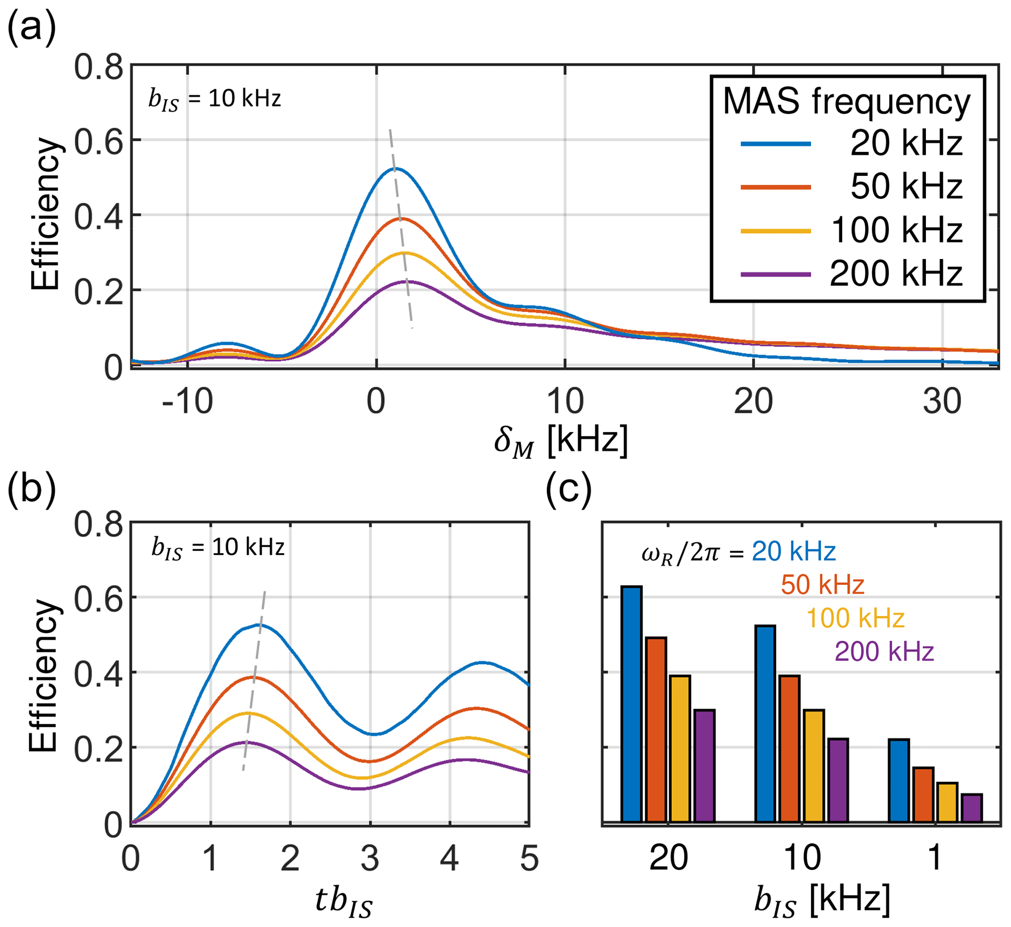
Figure 6Transfer efficiency of the constant amplitude CP experiment in the presence of RF field inhomogeneity and assuming a dipolar coupling strength bIS = 10 kHz. For the calculation, a rotor fully packed with material is assumed. (a) The maximum of the CP matching profile decreases with increasing MAS frequency for the zero-quantum () condition. At the same time, the width increases. A dashed gray line is used to indicate the position of the maximum. The maximum of the CP matching profile shifts to higher mismatch values δM for increased MAS frequencies. (b) Magnetization buildup curves for different MAS frequencies. The legend is indicated in panel (a). With increasing MAS frequencies, magnetization reaches the maximum transfer at shorter mixing times. (c) Maximum transfer efficiencies for the characteristic dipolar coupling values bIS of 1, 10 and 20 kHz for different MAS frequencies. Data were generated using Eqs. (27), (31) and (32).
We used numerical simulations in SIMPSON (Bak et al., 2000; Tošner et al., 2014) to verify the predictions of the analytical model. To implement an experiment, specific values of ωI and ωS need to be selected. A consideration of RF field inhomogeneity increases the complexity of this selection process, since certain values of ωI and ωS can lead to a situation in which ZQ and DQ recoupling conditions are fulfilled simultaneously in different parts of the sample (Fig. 4c). This phenomenon was explored experimentally by Gupta et al. (2015). If this situation is avoided, we find perfect agreement between the analytical model and the numerical simulations.
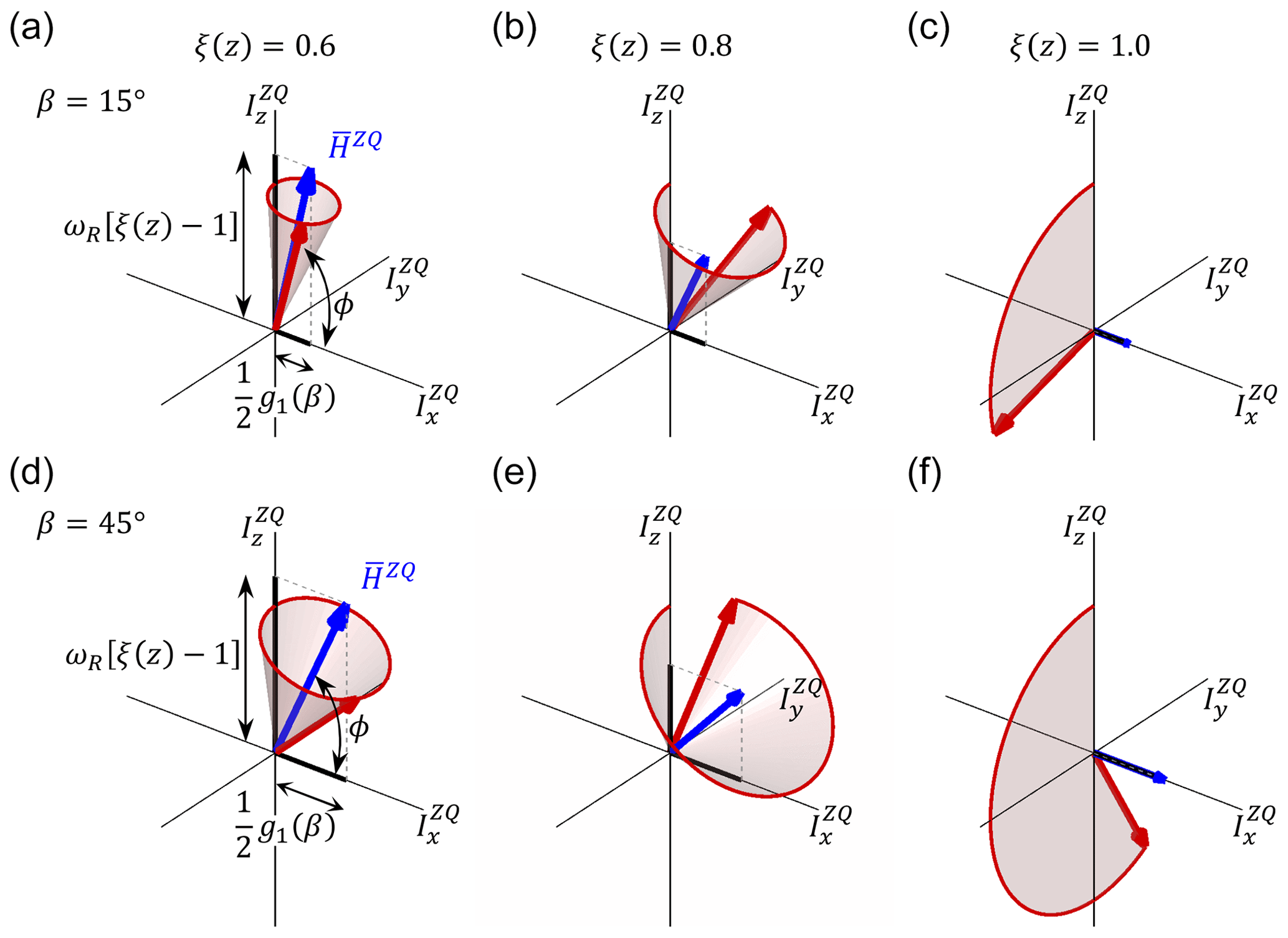
Figure 7Visualization of the spin state trajectories for the constant amplitude cross-polarization experiment evaluated for two crystal orientations. (a–c) Crystallite orientation β = 15∘; (d–f) β = 45∘. The calculations were carried out for three positions along the coil axis that correspond to RF field scaling values of ξ(z) = 0.6 (panels a and d), 0.8 (panels b and e) and 1.0 (panels c and f). The state vector, ρZQ, is represented by a red vector. The effective Hamiltonians are represented by blue vectors. ρZQ rotates around on the surface of a cone (shaded area). In the simulation, a MAS frequency of 50 kHz and bIS = 10 kHz was assumed.
3.2 Visualization of the magnetization transfer trajectories
In the following, we aim to visualize the spin trajectory during the CP experiment in its basic form with constant RF and with RF amplitude sweeps. We focus on the vicinity of the ZQ () Hartmann–Hahn condition and use the effective Hamiltonian given in Eq. (34) for the analysis. We consider RF field inhomogeneity and assume nominal RF amplitudes that match the recoupling condition in the center of the coil: . Figure 7 shows the spin dynamics for two crystallite orientations (β = 15 and 45∘) and three positions within the coil (ξ = 0.6, 0.8 and 1.0). These conditions are highlighted in Figs. 1 and 2. In the center of the coil where ξ = 1.0, the Hamiltonian (blue vector) is aligned with the axis. The spin state vector ρZQ(t) (red vector) rotates in circles within the yz plane with an angular velocity that depends on the crystallite orientation (Fig. 7c and f). This situation corresponds to the case without RF field inhomogeneity.
Depending on the position within the coil, a mismatch contribution in the effective Hamiltonian along the axis is obtained, which is according to Eq. (34) proportional to the MAS frequency. The effective rotation axis is tilted away from the direction by an angle ϕ (Eq. 23). The effective rotation frequency (Eq. 22) increases with increasing mismatch. Likewise, the component of decreases with the decreasing effective dipolar coupling. This amplifies the effect of the RF field inhomogeneity on the orientation of the effective Hamiltonian axis. The state vector rotates on the surface of a cone (Fig. 7a, b and d, e). As a consequence, the inversion becomes inefficient. Only the central part of the sample yields a high transfer efficiency.
3.3 RF amplitude sweeps in the absence of RF field inhomogeneity
Continuous RF amplitude sweeps are used to improve the cross-polarization efficiency. In this case, the effective Hamiltonian changes its orientation in the course of the pulse sequence. An adiabatic inversion is achieved if two conditions are fulfilled: (i) the initial state vector is aligned with the initial effective field vector and (ii) the effective field changes its orientation slowly. We focus on the zero-quantum () condition assuming a dipolar coupling constant bIS = 10 kHz. In the following, spin state trajectories are calculated for two sweep amplitudes: Δ = 10 and 30 kHz.
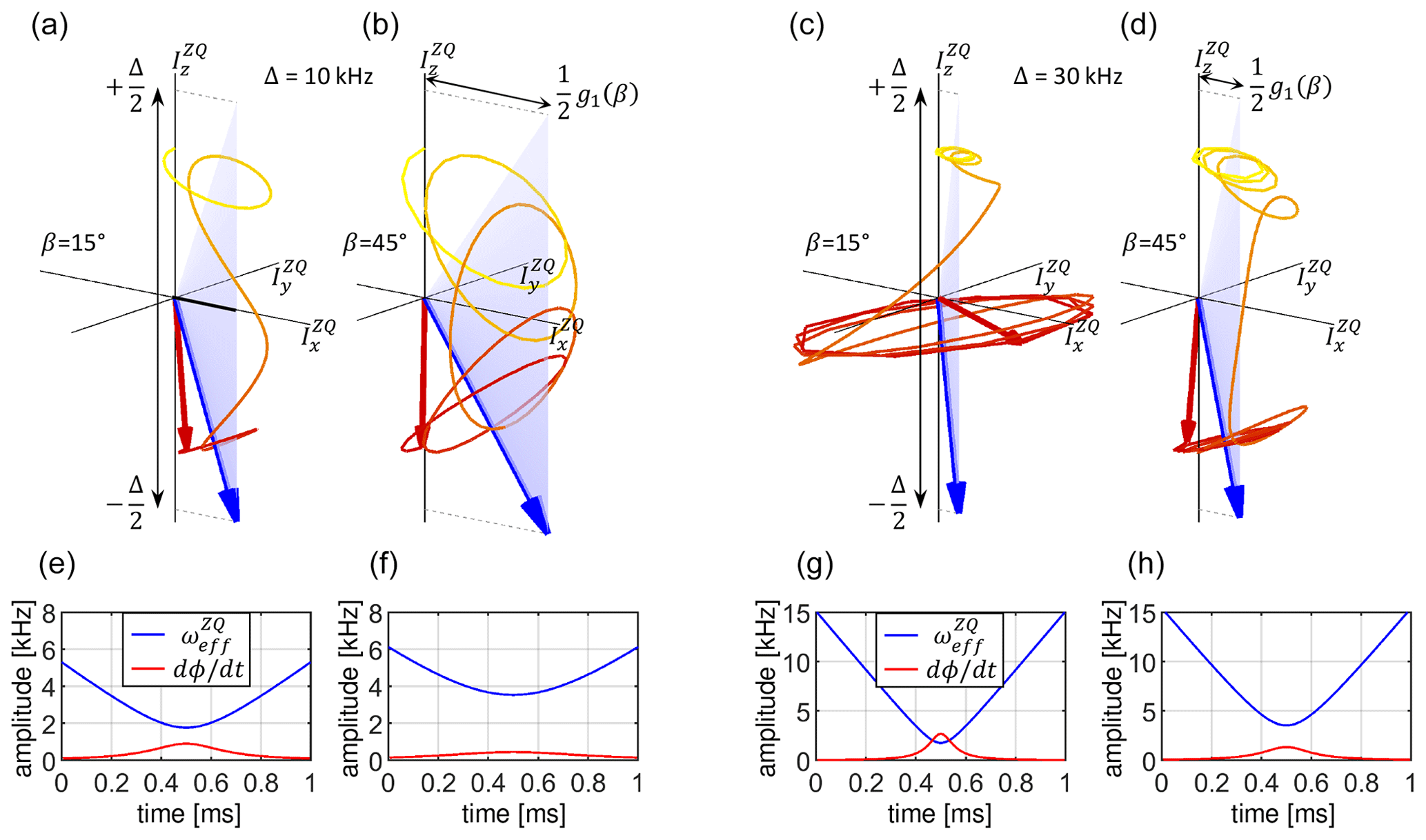
Figure 8Visualization of the spin state trajectories for the linear ramp cross-polarization experiment assuming a homogeneous RF field distribution. For the simulation, a dipolar coupling bIS = 10 kHz was assumed. The CP contact time was set to T = 1 ms. The calculation was carried out for two crystallite orientations (β = 15 and 45∘; panels a, c and b, d, respectively) and two sweep amplitudes (Δ = 10 kHz and Δ = 30 kHz; panels a, b and c, d, respectively). The blue-shaded areas represent the changing effective Hamiltonian. The blue arrow indicates the effective Hamiltonian at the end of the pulse sequence at t=T. The component along the axis is time dependent, while the axis component is fixed (see Eq. 40). The beginning of the trajectory is depicted as a yellow line which gradually turns red as the trajectory progresses. The final state of the spin state vector (initially oriented along ) is drawn as a red arrow. Panels (e–h) display and . In (c, g), the adiabaticity condition is violated during the sweep.
The spin state trajectories for the linear ramp are represented in Fig. 8. The component of the effective Hamiltonian is fixed in time and is given by the effective dipolar coupling at a given orientation (Eq. 40, assuming ξ = 1.0). The maximal value of is reached for β = 45∘, which together with the sweep amplitude of Δ = 10 kHz and according to Eq. (23) results in a tilt angle of the effective field = 54.7∘ at the beginning of the pulse sequence (Fig. 8b). Clearly, the initial state vector is not aligned with the effective field of . However, the inversion efficiency is high due to the slow change in the orientation of the effective field, , such that the state vector can follow the effective field while it is rotating around it in rather large circles (see evaluation of the adiabaticity condition in Fig. 8f). For a smaller effective dipolar coupling (for example, β = 15∘ in Fig. 8a), the angle ϕ is larger (close to 90∘). During the linear ramp, the effective Hamiltonian amplitude goes through a minimum in the middle of the sweep at , where its value is solely determined by the effective dipolar coupling; see Eq. (22). At the same time, reaches its maximum (Fig. 8e). Under these conditions, the state vector keeps track of the effective field (Fig. 8a). When a larger sweep amplitude is employed, e.g., Δ = 30 kHz, the orientation of the initial effective field is closer to the axis, = 76.7∘ (Fig. 8d). At the same time, the amplitude of the effective Hamiltonian is increased as well. For the crystallite orientation β = 15∘ (Fig. 8c), however, we find that the adiabaticity condition is violated in the middle of the pulse sequence (Fig. 8g). The state vector is not able to follow the effective field as becomes too high. As a consequence, the state vector keeps rotating near the Equator (Fig. 8c) and thus contributes little to the total transfer efficiency.
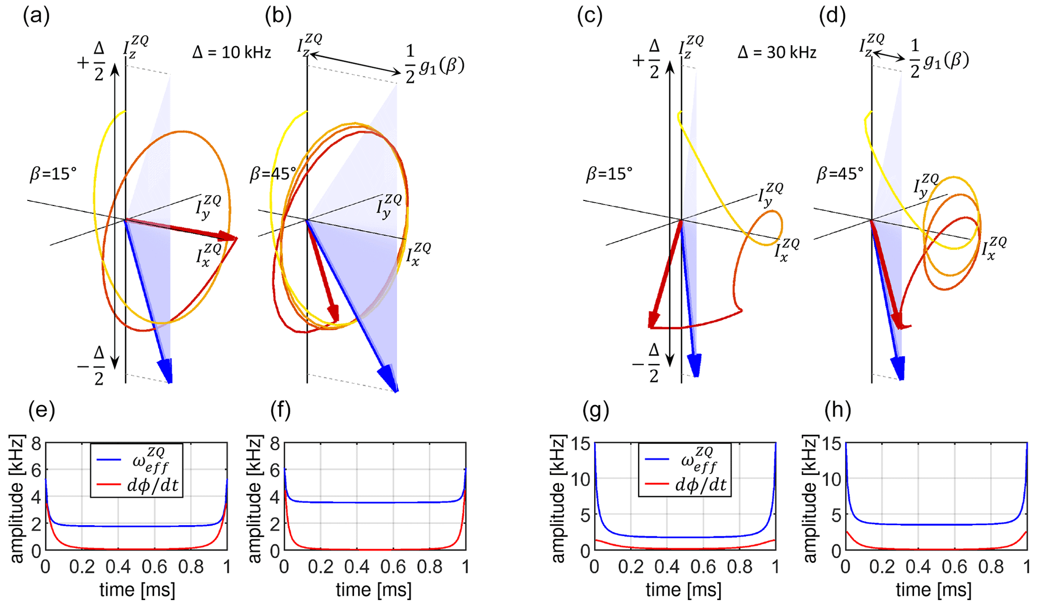
Figure 9Visualization of the spin state trajectories for the adiabatic tangential sweep cross-polarization experiment assuming a homogeneous RF field distribution. For the simulation, a dipolar coupling bIS = 10 kHz was assumed. The CP contact time was set to T = 1 ms. The calculation was carried out for two crystallite orientations (β = 15 and 45∘; panels a, c and b, d, respectively) and two sweep amplitudes (Δ = 10 kHz and Δ = 30 kHz; panels a, b and c, d, respectively, . The blue-shaded areas represent the changing effective Hamiltonian. The blue arrow indicates the effective Hamiltonian at the end of the pulse sequence at t=T. The component along the axis is time dependent, while the axis component is fixed (see Eq. 40). The beginning of the trajectory is depicted as a yellow line which gradually turns red as the trajectory progresses. The final state of the spin state vector (initially oriented along ) is drawn as a red arrow. Panels (e–h) display and . In (a, e) and (b, f), the adiabaticity condition <ωeff is violated during the sweep.
Spin state trajectories for the adiabatic variant of the CP experiment are shown in Fig. 9. The tangential sweep has been suggested to keep the rate of change small compared to the effective field amplitude at all times (Hediger et al., 1995). Initially, ωeff(t) is large implying that can be large. However, for small sweep amplitudes such as Δ = 10 kHz, the effective field changes too rapidly for a portion of crystallites at the beginning and at the end of the sweep so that the adiabaticity condition is violated (Fig. 9e). Most of the dynamics take place when the tangential function goes through the central plateau, where the RF amplitudes do not change significantly over an extended period of time. The state vector rotates in large circles around the effective Hamiltonian that is oriented predominantly along the axis. When a larger sweep amplitude Δ = 30 kHz is used, the adiabatic regime is restored for most crystallite orientations and an improved transfer efficiency is obtained.
Figure 10 compares the magnetization transfer during the RF sweep for the examples discussed above. The transfer process is fast when the change in the effective field orientation is fast: in the middle of the linear ramp and at the beginning and at the end of the tangential sweep, provided the adiabaticity condition is maintained (Fig. 10a and b). Figure 10c and d shows the transfer efficiency as a function of crystallite orientation. Note that the spin state inversion cannot be achieved for crystallite orientations with an effective dipolar coupling that is vanishing, i.e., for β = 0 and 90∘. The portion of crystallites yielding low transfer depends on the ratio of the sweep amplitude Δ and the dipolar coupling bIS. For the linear ramp, Δ = 10 kHz is preferable, while the tangential sweep using an amplitude Δ = 30 kHz yields high efficiency for most of the crystallites under the conditions investigated here. After powder averaging, the magnetization transfer efficiency is on the order of 90 % for the tangential sweep. We would like to note that all predictions based on the ZQ average Hamiltonian agree well with exact simulations using SIMPSON.
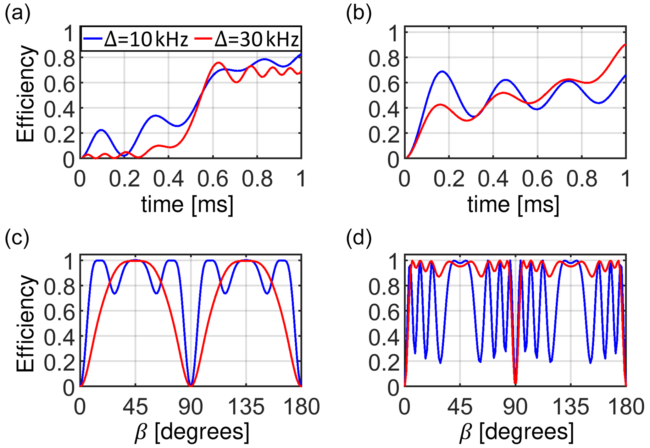
Figure 10Powder-averaged buildup of the transferred magnetization during the mixing time of the CP experiment (a, b) and the final transfer efficiency as a function of crystallite orientation (c, d) for an RF amplitude sweep using a linear ramp (a, c) and a tangential shape (b, d). The blue and red curves correspond to sweep amplitudes of 10 and 30 kHz, respectively. In all simulations, a homogeneous RF field distribution is assumed.
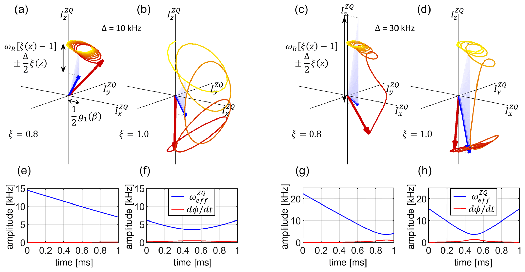
Figure 11Visualization of the spin state trajectory for a linear ramp cross-polarization experiment assuming an inhomogeneous RF field distribution. For the simulation, a dipolar coupling bIS = 10 kHz was assumed. The CP contact time was set to T = 1 ms. The calculation was carried out for one crystallite orientation (β = 45∘) and two positions along the coil axis with RF field scaling factors ξ = 0.8 and 1.0 (panels a, c and b, d) and two sweep amplitudes Δ = 10 kHz and Δ = 30 kHz (panels a, b and c, d). The blue-shaded areas represent the changing effective Hamiltonian. The blue arrow indicates the effective Hamiltonian at the end of the pulse sequence at t=T. The component along the axis is time dependent, while the axis component is fixed (see Eq. 40). The beginning of the trajectory is depicted as a yellow line which gradually turns red as the trajectory progresses. The final state of the spin state vector (initially oriented along ) is drawn as a red arrow. Panels (e–h) display and to appreciate whether the adiabaticity condition <ωeff is violated during the sweep.
3.4 RF amplitude sweeps in the presence of an inhomogeneous RF field
In the following paragraph, RF field inhomogeneities are included in the analysis. For simplicity, we assume that the RF field varies along the solenoid coil axis as described in Fig. 2 and the variation is the same for both RF channels. We disregard time modulations induced by sample rotation in a spatially inhomogeneous RF field. We assume that the Hartmann–Hahn condition is fulfilled for the nominal RF amplitudes in the middle of the coil. The RF amplitude sweep is applied to the I channel. We again examine the zero-quantum () recoupling condition. The drive Hamiltonian is given by Eq. (40). Sweeping the RF amplitude makes the component of the effective Hamiltonian time dependent. The range over which it varies depends on the position along the coil axis, and it is visualized in Fig. 4. The center of the sweep is shifted away from the exact matching condition towards the ends of the coil by an amount that depends on the MAS frequency. As discussed above, the evolution in the double-quantum subspace can be neglected, since has a dominant component along axis which is much larger than the effective dipolar coupling. This can be achieved by choosing a proper value for . At the same time, we have chosen conditions that avoid simultaneous matching of different Hartmann–Hahn conditions within the sample volume.
The previous description of the RF-amplitude-modulated CP is valid at the center of the coil where ξ = 1.0. The situation is quite different in volume elements towards the ends of the coil. Figure 11 illustrates the spin state trajectories for the linear ramp CP experiment, assuming a crystallite angle β = 45∘, a MAS frequency of = 50 kHz and a dipolar coupling constant of bIS = 10 kHz. The scaling factor ξ = 0.8 is realized for (where l is the coil length) around the center of the coil. When the sweep amplitude is Δ = 10 kHz, the effective field does not get inverted during the sweep (Figs. 4a and 11a) and therefore cannot invert the spin state, regardless of its adiabaticity (Fig. 11e). Increasing the sweep amplitude to Δ = 30 kHz yields better results as the effective field approaches the Hartmann–Hahn recoupling condition towards the end of the sweep period (Figs. 4b and 11c).
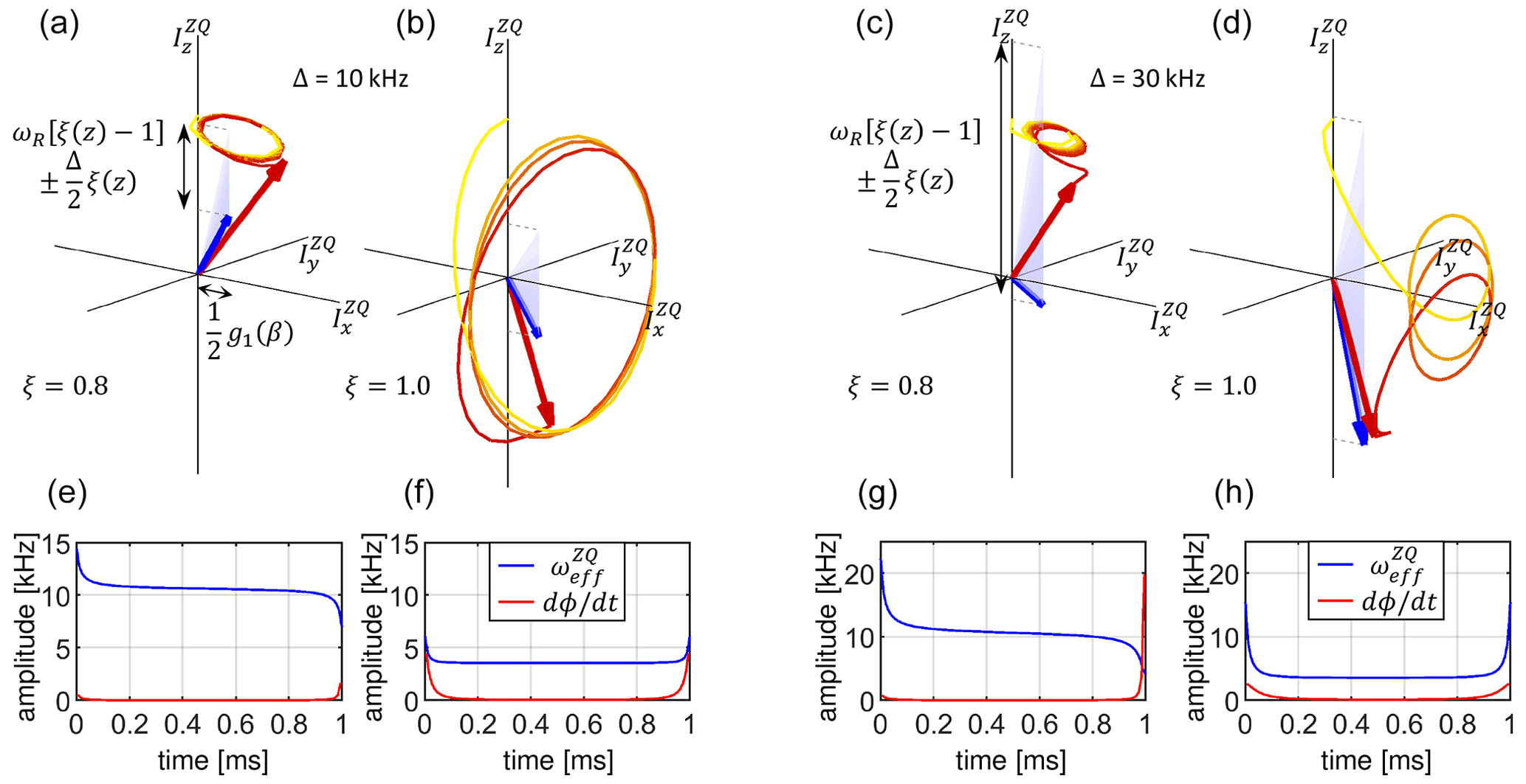
Figure 12Visualization of the spin state trajectory for an adiabatic tangential sweep cross-polarization experiment assuming an inhomogeneous RF field. For the simulation, a dipolar coupling bIS = 10 kHz was assumed. The CP contact time was set to T = 1 ms. The calculation was carried out for one crystallite orientation (β = 45∘) and two positions along the coil axis with RF field scaling factors ξ = 0.8 and 1.0 (panels a, c and b, d) and two sweep amplitudes Δ = 10 kHz and Δ = 30 kHz, assuming (panels a, b and c, d). The blue-shaded areas represent the changing effective Hamiltonian. The blue arrow indicates the effective Hamiltonian at the end of the pulse sequence at t=T. The component along the axis is time dependent, while the axis component is fixed (see Eq. 40). The beginning of the trajectory is depicted as a yellow line which gradually turns red as the trajectory progresses. The final state of the spin state vector (initially oriented along ) is drawn as a red arrow. Panels (e–h) display and to appreciate whether the adiabaticity condition <ωeff is violated during the sweep.
For a tangential sweep, the spin state trajectories are depicted in Fig. 12. Initially, and towards the end of the sweeping period, the RF amplitude changes rapidly and so does the effective field orientation. This can lead to a violation of the adiabaticity condition, as encountered for the calculation with a sweep amplitude of Δ = 30 kHz (Fig. 12c and g). Despite the fact that the Hartmann–Hahn matching condition is included within the sweep range, the state vector does not follow the effective field. These parts of the sample yield a low transfer efficiency.
The buildup of the transferred magnetization integrated over the sample volume and detected by the NMR coil for both the linear ramp and the tangential sweep is presented in Fig. 13a and b. It is not obvious which sweeping method will yield a higher total transfer efficiency. Of the four setups discussed so far, the linear ramp with Δ = 30 kHz yields the best result. When comparing efficiency profiles along the coil axis (Fig. 13c and d), we observe that a tangential sweep is more efficient near the center of the coil but quickly loses efficiency when going towards the ends. However, a linear ramp yields equal transfer over a larger sample volume.
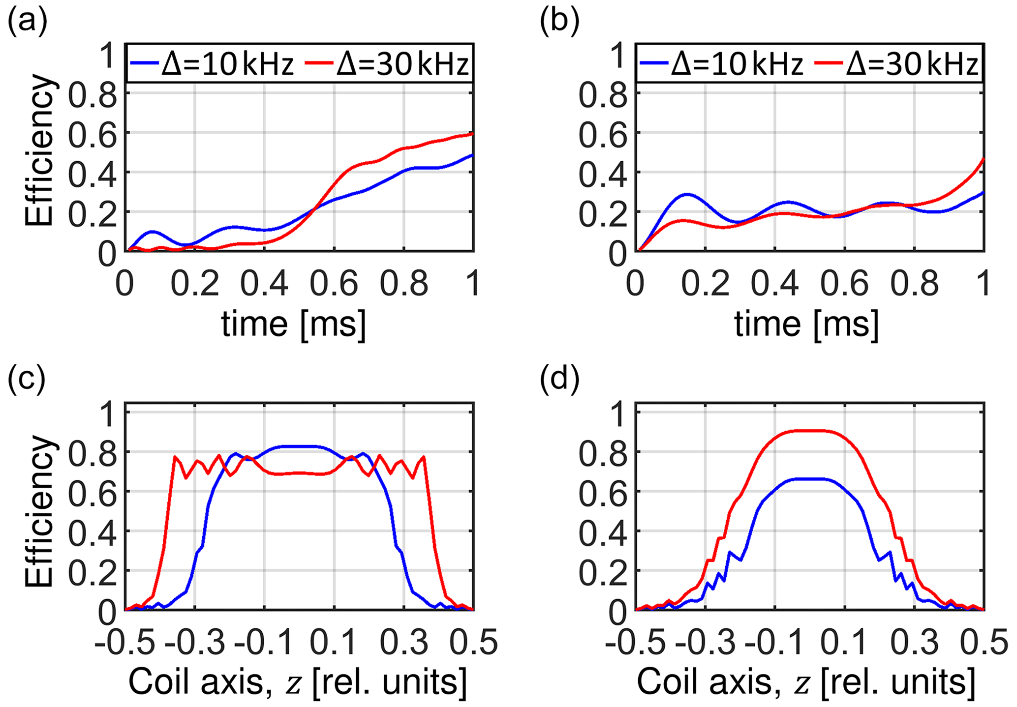
Figure 13Powder-averaged buildup of transferred magnetization during the mixing time of the CP experiment (a, b) and the final powder-averaged transfer efficiency as a function of the position along the coil axis (c, d) for a linear ramp (a, c) and a tangential shape (b, d). The blue and red curves correspond to sweep amplitudes of Δ = 10 kHz and Δ = 30 kHz, respectively. In the calculation, an inhomogeneous RF field is assumed.
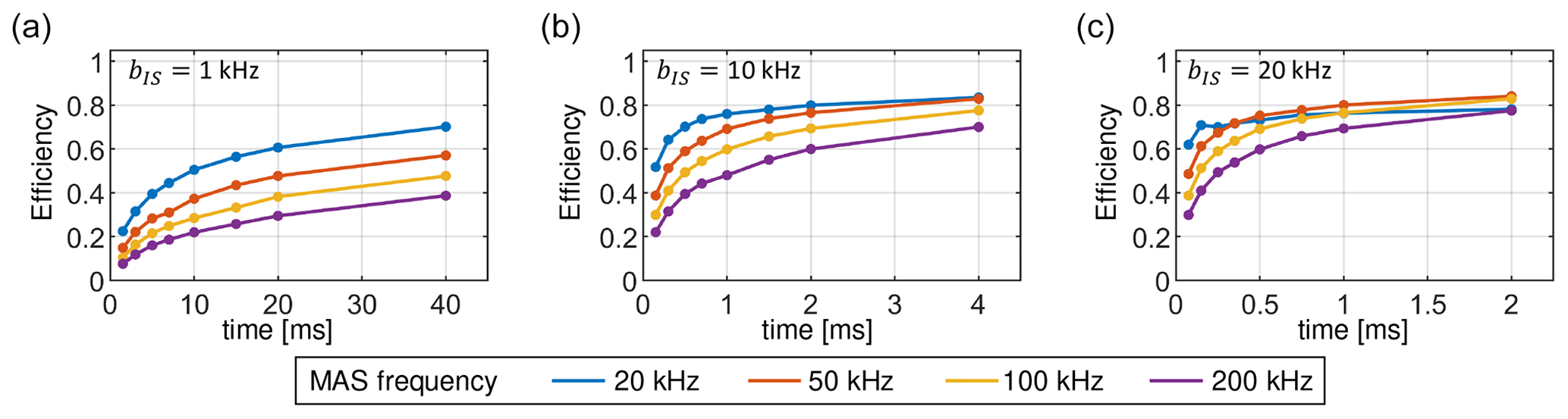
Figure 14Maximum achievable transfer efficiencies in the cross-polarization experiment as a function of contact time and MAS frequency using numerical optimizations. Similar efficiencies are obtained for both the linear ramp and the tangential sweep, although different shape parameters have to be employed. Dipolar couplings of 1, 10 and 20 kHz are used in the simulations for panels (a–c), respectively.
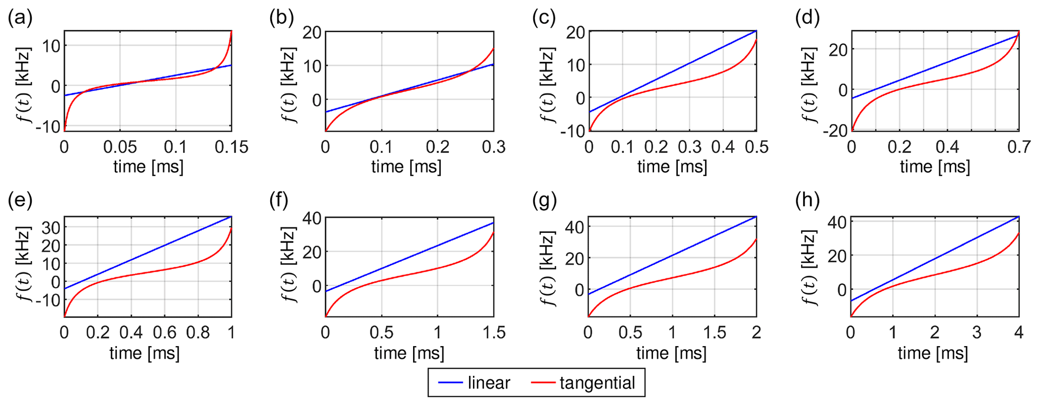
Figure 15Comparison of optimal linear ramp (blue) and tangential sweep (red) shapes obtained by numerical optimizations at different contact times T = 0.15, 0.3, 0.5, 0.7, 1.0, 1.5, 2.0 and 4.0 ms in panels (a–h), respectively. For the optimization, a dipolar coupling bIS = 10 kHz was assumed. The calculations were performed assuming a MAS frequency of 50 kHz and a realistic RF inhomogeneity distribution. Although the two shapes are different, they yield virtually identical total transfer efficiencies.
3.5 Numerical optimizations of linear and tangential sweeps
In this section, we discuss which parameters of a linear ramp and a tangential sweep yield the best transfer efficiency. We address this problem by a numerical optimization. The calculations are repeated for a range of dipolar couplings and MAS frequencies. In the case of the linear ramp, the sweep amplitude Δ and the offset δM from the exact Hartmann–Hahn condition are optimized. In the case of the tangential sweep, the curvature parameter b is considered in addition (Fig. 3). The offset parameter δM corresponds to the mismatch of the recoupling condition in the middle of the coil due to RF inhomogeneity and reflects the experimental optimization procedure where the amplitude is kept constant and the amplitude is optimized around the expected recoupling condition. To ensure that no more than one matching condition is encountered during the sweep, the amplitude Δ was restricted to values within ± (Hediger et al., 1995). The dynamics were evaluated using the effective Hamiltonian given in Eq. (40). The optimized parameters correspond to the best transfer efficiency obtained from 100 repetitions initiated by random guess. As expected, we obtain a different set of optimal parameters for each contact time, dipolar coupling and MAS frequency.
The optimized transfer efficiencies are summarized in Fig. 14. Remarkably, we have not found any significant differences in the performance of the linear ramp with respect to the tangential sweep. Both sweep methods yield the same total transfer efficiency, although they use different sweep parameters. An example of the best sweep shapes obtained for a dipolar coupling bIS = 10 kHz and a MAS frequency of 50 kHz is presented in Fig. 15. The tangential sweeps tend to have a larger sweep amplitude Δ and a smaller offset values δM when compared to the linear ramp.
We observe that very long contact times are required to obtain high transfer efficiencies. For calculations involving different dipolar coupling strengths bIS the same range of the reduced time parameter TbIS is used. In this way, longer mixing times T are maintained for smaller dipolar couplings bIS. Better performance is obtained for cases with higher dipolar couplings, which correlates with the width of Hartmann–Hahn conditions in CP matching profiles. On the other hand, the transfer efficiency decreases at higher MAS frequencies due to increased volume selectivity. Small dipolar couplings are the most challenging, on the order of 1 kHz, and ultrafast MAS (> 100 kHz), which are typical of 15N–13C spin pairs in proteins studied by proton-detected MAS solid-state NMR experiments. To more efficiently average proton dipolar interaction, MAS probe development aims at smaller-diameter rotors to achieve higher MAS rotation frequencies. Currently, 0.4 mm MAS probes are in development that can reach MAS frequencies of up to 200 kHz. Our predictions suggest that only 20 % of the sample will contribute to the detected NMR signal after a 10 ms 15N–13C CP mixing step at a MAS frequency of 200 kHz; i.e., up to 80 % of the signal is lost in a single magnetization transfer step. The efficiency increases to ca. 40 % when a 40 ms long mixing period is used, provided that there are no signal losses due to relaxation. However, note that the sensitivity in a pulse sequence with multiple CP transfer elements depends on all previous transfer steps. The first CP element preselects a volume that is maintained or further restricted in subsequent transfer elements.
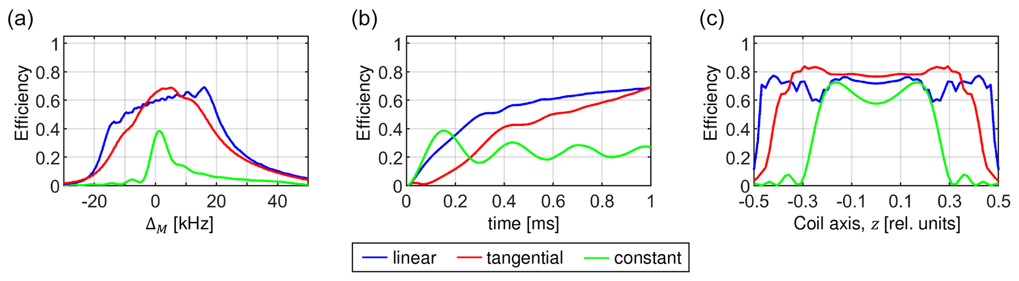
Figure 16Comparison of the matching profiles (a), magnetization transfer buildups (b) and contribution to the transfer efficiency of individual volume elements along the coil axis (c) for an optimized linear ramp (blue), a tangential sweep (red) and a constant amplitude CP (green). For the optimization, a dipolar coupling bIS = 10 kHz was assumed. The calculations were performed assuming a MAS frequency of 50 kHz and a realistic RF inhomogeneity distribution. The CP contact time was set to T = 1 ms. In (a) and (c), the constant amplitude CP was evaluated after 160 µs when it reaches maximum transfer efficiency.
We find that there is no difference between the linear ramp and the tangential shapes in terms of total transfer efficiency. In Fig. 16, we compare these two methods (together with a constant amplitude CP) with respect to the width of the CP matching profile (Fig. 16a), the magnetization transfer buildup (Fig. 16b) and the sample volume selectivity (Fig. 16c). As expected, the RF amplitude sweep significantly improves the width and the height of the matching profile. The most important difference is that the tangential sweep yields higher efficiency near the center of the coil and lower efficiency at edges of the coil. Use of RF pulses and other recoupling elements can potentially result in a preselection of a particular sample volume that cannot be utilized by the linear ramp for a further transfer. Therefore, transfer elements should be optimized within the framework of the whole pulse sequence to minimize a differential preselection of the sample volume during calibration experiments.
The linear ramp and the adiabatic tangential sweeps were calculated for the ZQ () condition. However, the shapes are equally applicable to any other n = ± 1 Hartmann–Hahn condition, as the corresponding effective Hamiltonian has the same form. The n = ± 2 Hartmann–Hahn conditions suffer from increased RF field inhomogeneity (factor of 2 in Eq. 40) and have different powder averaging properties implied by the g2(β) term. Thus, a decreased CP transfer efficiency for the n = ± 2 matching condition is expected.
The transfer efficiencies of all pulse sequences were verified using numerical simulations in SIMPSON. To avoid overlap of the different Hartmann–Hahn matching conditions, the zero-quantum () condition with = 60 kHz was selected using MAS frequencies of 20 and 50 kHz, while the double-quantum () condition with = 30 kHz was used for a MAS frequency of 100 kHz. The agreement between SIMPSON and the effective Hamiltonian calculations is excellent except for a simulation in which a dipolar coupling of 20 kHz and a MAS frequency of 20 kHz was assumed. In this case, the numerically evaluated transfer efficiencies are about 10 % lower. A plausible explanation is that the first-order average Hamiltonian approximation does not provide the full description of the spin dynamics when the dipolar coupling and the MAS frequency are of similar value (in other cases it holds .
We have analyzed the magnetization transfer efficiency of the CP experiment as a function of the MAS frequency in the presence of RF field inhomogeneity of a solenoid coil. We show that a sweep of the RF amplitude through the Hartmann–Hahn matching conditions using either a linear ramp or a tangential shape improves the performance in a comparable way. We do not observe a difference in the total transfer efficiency between these two methods. We find that magnetization transfer using a CP recoupling element becomes inefficient in particular for small dipolar couplings for ultrafast MAS experiments with rotation frequencies above 100 kHz. New recoupling methods that are designed explicitly to account for inhomogeneous RF fields and ultrafast MAS conditions are needed to overcome this issue in the future.
No data sets were used in this article.
ZT and BR conceived the project. AŠ carried out numerical calculations. JB, AŠ, BR and ZT discussed the results, outlined the paper and collaborated on the final text. ZT wrote the paper.
At least one of the (co-)authors is a member of the editorial board of Magnetic Resonance. The peer-review process was guided by an independent editor, and the authors also have no other competing interests to declare.
Publisher's note: Copernicus Publications remains neutral with regard to jurisdictional claims in published maps and institutional affiliations.
This research has been supported by a joint project between the Czech Science Foundation (20-00166J, ZT) and Deutsche Forschungsgemeinschaft (Re 1435/20-1, BR).
This work was supported by the Technical University of Munich (TUM) in the framework of the Open Access Publishing Program.
This paper was edited by Perunthiruthy Madhu and reviewed by three anonymous referees.
Aebischer, K., Tošner, Z., and Ernst, M.: Effects of radial radio-frequency field inhomogeneity on MAS solid-state NMR experiments, Magn. Reson., 2, 523–543, https://doi.org/10.5194/mr-2-523-2021, 2021.
Andrew, E. R., Bradbury, A., and Eades, R. G.: Nuclear Magnetic Resonance Spectra from a Crystal rotated at High Speed, Nature, 182, 1659–1659, https://doi.org/10.1038/1821659a0, 1958.
Bak, M., Rasmussen, J. T., and Nielsen, N. C.: SIMPSON: A general simulation program for solid-state NMR spectroscopy, J. Magn. Reson., 147, 296–330, https://doi.org/10.1006/jmre.2000.2179, 2000.
Baum, J., Tycko, R., and Pines, A.: Broadband and adiabatic inversion of a two-level system by phase-modulated pulses, Phys. Rev. A (Coll Park), 32, 3435–3447, https://doi.org/10.1103/PhysRevA.32.3435, 1985.
Brinkmann, A.: Introduction to average Hamiltonian theory. I. Basics, Concep. Magn. Reson. A, 45A, e21414, https://doi.org/10.1002/cmr.a.21414, 2016.
Engelke, F.: Electromagnetic wave compression and radio frequency homogeneity in NMR solenoidal coils: Computational approach, Concept. Magnetic. Res., 15, 129–155, https://doi.org/10.1002/cmr.10029, 2002.
Gupta, R., Hou, G., Polenova, T., and Vega, A. J.: RF inhomogeneity and how it controls CPMAS, Solid State Nucl Mag., 72, 17–26, https://doi.org/10.1016/j.ssnmr.2015.09.005, 2015.
Hartmann, S. R. and Hahn, E. L.: Nuclear Double Resonance in the Rotating Frame, Phys. Rev., 128, 2042–2053, 1962.
Hassan, A., Quinn, C. M., Struppe, J., Sergeyev, I. V., Zhang, C., Guo, C., Runge, B., Theint, T., Dao, H. H., Jaroniec, C. P., Berbon, M., Lends, A., Habenstein, B., Loquet, A., Kuemmerle, R., Perrone, B., Gronenborn, A. M., and Polenova, T.: Sensitivity boosts by the CPMAS CryoProbe for challenging biological assemblies, J. Magn. Reson., 311, 106680, https://doi.org/10.1016/j.jmr.2019.106680, 2020.
Hediger, S., Meier, B. H., and Ernst, R. R.: Adiabatic passage hartmann-hahn cross-polarization in nmr under magic-angle sample-spinning, Chem. Phys. Lett., 240, 449–456, https://doi.org/10.1016/0009-2614(95)00505-x, 1995.
Hoult, D. I.: The principle of reciprocity in signal strength calculations – A mathematical guide, Concept. Magnetic. Res., 12, 173–187, https://doi.org/10.1002/1099-0534(2000)12:4<173::aid-cmr1>3.0.co;2-q, 2000.
Idziak, S. and Haeberlen, U.: Design and construction of a high homogeneity rf coil for solid-state multiple-pulse NMR, J. Magn. Reson., 50, 281–288, https://doi.org/10.1016/0022-2364(82)90058-0, 1982.
Kelz, J. I., Kelly, J. E., and Martin, R. W.: 3D-printed dissolvable inserts for efficient and customizable fabrication of NMR transceiver coils, J. Magn. Reson., 305, 89–92, https://doi.org/10.1016/j.jmr.2019.06.008, 2019.
Krahn, A., Priller, U., Emsley, L., and Engelke, F.: Resonator with reduced sample heating and increased homogeneity for solid-state NMR, J. Magn. Reson., 191, 78–92, https://doi.org/10.1016/j.jmr.2007.12.004, 2008.
Laage, S., Sachleben, J. R., Steuernagel, S., Pierattelli, R., Pintacuda, G., and Emsley, L.: Fast acquisition of multi-dimensional spectra in solid-state NMR enabled by ultra-fast MAS, J. Magn. Reson., 196, 133–141, https://doi.org/10.1016/j.jmr.2008.10.019, 2009.
Levitt, M. H.: Heteronuclear cross polarization in liquid-state nuclear magnetic resonance: Mismatch compensation and relaxation behavior, J. Chem. Phys., 94, 30–38, https://doi.org/10.1063/1.460398, 1991.
Lowe, I. J.: Free Induction Decays of Rotating Solids, Phys. Rev. Lett., 2, 285–287, https://doi.org/10.1103/PhysRevLett.2.285, 1959.
Marica, F. and Snider, R. F.: An analytical formulation of CPMAS, Solid State Nucl Mag., 23, 28–49, https://doi.org/10.1016/S0926-2040(02)00013-9, 2003.
Marks, D. and Vega, S.: A Theory for Cross-Polarization NMR of Nonspinning and Spinning Samples, J. Magn. Reson. Ser. A, 118, 157–172, https://doi.org/10.1006/jmra.1996.0024, 1996.
Meier, B. H.: Cross polarization under fast magic angle spinning: thermodynamical considerations, Chem. Phys. Lett., 188, 201–207, https://doi.org/10.1016/0009-2614(92)90009-C, 1992.
Metz, G., Wu, X. L., and Smith, S. O.: Ramped-amplitude cross-polarization in magic-angle-spinning NMR, J. Magn. Reson. Ser. A, 110, 219–227, https://doi.org/10.1006/jmra.1994.1208, 1994.
Paulson, E. K., Martin, R. W., and Zilm, K. W.: Cross polarization, radio frequency field homogeneity, and circuit balancing in high field solid state NMR probes, J. Magn. Reson., 171, 314–323, https://doi.org/10.1016/j.jmr.2004.09.009, 2004.
Peersen, O. B., Wu, X. L., and Smith, S. O.: Enhancement of CP-MAS Signals by Variable-Amplitude Cross Polarization. Compensation for Inhomogeneous B1 Fields, J. Magn. Reson. Ser. A, 106, 127–131, https://doi.org/10.1006/jmra.1994.1014, 1994.
Pines, A., Gibby, M. G., and Waugh, J. S.: Proton-enhanced NMR of dilute spins in solids, J. Chem. Phys., 59, 569–590, https://doi.org/10.1063/1.1680061, 1973.
Privalov, A. F., Dvinskikh, S. V, and Vieth, H. M.: Coil design for large-volume high-B-1 homogeneity for solid-state NMR applications, J. Magn. Reson. Ser. A, 123, 157–160, https://doi.org/10.1006/jmra.1996.0229, 1996.
Ray, S., Ladizhansky, V., and Vega, S.: Simulation of CPMAS signals at high spinning speeds, J. Magn. Reson., 135, 427–434, https://doi.org/10.1006/jmre.1998.1562, 1998.
Rovnyak, D.: Tutorial on analytic theory for cross-polarization in solid state NMR, Concep. Magn. Reson. A, 32A, 254–276, https://doi.org/10.1002/cmr.a.20115, 2008.
Schaefer, J.: A Brief History of the Combination of Cross Polarization and Magic Angle Spinning, in: Encyclopedia of Magnetic Resonance, John Wiley & Sons, Ltd, Chichester, UK, https://doi.org/10.1002/9780470034590.emrhp0161, 2007.
Stejskal, E. O., Schaefer, J., and Waugh, J. S.: Magic-angle spinning and polarization transfer in proton-enhanced NMR, J. Magn. Reson. (1969), 28, 105–112, https://doi.org/10.1016/0022-2364(77)90260-8, 1977.
Tošner, Z., Andersen, R., Stevenss, B., Eden, M., Nielsen, N. C., Vosegaard, T., Stevensson, B., Eden, M., Nielsen, N. C., and Vosegaard, T.: Computer-intensive simulation of solid-state NMR experiments using SIMPSON, J. Magn. Reson., 246, 79–93, https://doi.org/10.1016/j.jmr.2014.07.002, 2014.
Tošner, Z., Purea, A., Struppe, J. O., Wegner, S., Engelke, F., Glaser, S. J., and Reif, B.: Radiofrequency fields in MAS solid state NMR probes, J. Magn. Reson,, 284, 20–32, https://doi.org/10.1016/j.jmr.2017.09.002, 2017.
Tošner, Z., Sarkar, R., Becker-Baldus, J., Glaubitz, C., Wegner, S., Engelke, F., Glaser, S. J., and Reif, B.: Overcoming Volume Selectivity of Dipolar Recoupling in Biological Solid-State NMR Spectroscopy, Angew. Chem. Int. Edit., 57, 14514–14518, https://doi.org/10.1002/anie.201805002, 2018.
Wu, X. L. and Zilm, K. W.: Cross Polarization with High-Speed Magic-Angle Spinning, J. Magn. Reson. Ser. A, 104, 154–165, https://doi.org/10.1006/jmra.1993.1203, 1993.