the Creative Commons Attribution 4.0 License.
the Creative Commons Attribution 4.0 License.
 | 05 Jun 2023
The solid effect of dynamic nuclear polarization in liquids
The solid-state effect of dynamic nuclear polarization (DNP) is operative also in viscous liquids where the dipolar interaction between the electronic and nuclear spins is partially averaged. The proper way to quantify the degree of averaging, and thus calculate the efficiency of the effect, should be based on the time-correlation function of the dipolar interaction. Here we use the stochastic Liouville equation formalism to develop a general theoretical description of the solid effect in liquids. The derived expressions can be used with different dipolar correlations functions depending on the assumed motional model. At high magnetic fields, the theory predicts DNP enhancements at small offsets, far from the classical solid-effect positions that are displaced by one nuclear Larmor frequency from the electronic resonance. The predictions are in quantitative agreement with such enhancement peaks observed at 9.4 T (Kuzhelev et al., 2022). These non-canonical peaks are not due to thermal mixing or the cross effect but exactly follow the dispersive component of the EPR line.
- Article
(5061 KB) - Full-text XML
- Companion paper
- BibTeX
- EndNote


The last 2 decades have witnessed an overarching development in nuclear hyperpolarization techniques across the entire spectrum of mechanisms, from the classical Overhauser and solid-state effects to (photo)chemically induced and parahydrogen-based polarization (Eills et al., 2023). While the majority of the reported applications have relied on polarization transfer in the solid state at cryogenic temperatures (Ni et al., 2013; Pinon et al., 2021), transfer in the liquid state at elevated (room or physiological) temperatures has also been actively explored (Prisner et al., 2016; Denysenkov et al., 2022). In the liquid state, the mechanism of polarization has almost exclusively been the Overhauser effect (Jakdetchai et al., 2014). One notable exception is the work of Stapf and coworkers in which the solid effect of dynamic nuclear polarization (DNP) has been employed in combination with field-cycling relaxometry to characterize the molecular dynamics in ionic liquids and polymer melts at ambient temperatures (Neudert et al., 2017; Gizatullin et al., 2019, 2021a, b, 2022).
At X band (9.6 GHz/0.35 T), where the DNP measurements of Stapf and colleagues have been carried out, the nuclear Larmor frequencies of 1H and 19F (ωI≈15 MHz) are less than the EPR spectral width of a nitroxide free radical and even comparable to the spectral width of the single-line radical BDPA (Gizatullin et al., 2021b). As a result, the negative and positive solid-effect enhancements overlap and partly cancel each other, complicating the quantitative analysis of the effect. An additional difficulty for quantification is that, in many instances, the Overhauser and solid effects coexist (Leblond et al., 1971b; Neudert et al., 2017; Gizatullin et al., 2022). Although the contributions of these two effects can generally be distinguished on the basis of their even (Overhauser effect) and odd (solid effect) parity with the offset from the electronic resonance, this identification could be complicated when the EPR spectrum is broad and asymmetrical.
To quantify the field profile of the DNP enhancement (i.e., the DNP spectrum), Stapf and colleagues use a weighted sum of (i) the EPR line shape (for the Overhauser effect) and (ii) the same line shape shifted by ±ωI, with one of the shifted copies flipped around the vertical axis (for the solid effect) (Neudert et al., 2017; Gizatullin et al., 2021b). The relative contribution of the two effects is then treated as a fitting parameter. In general, the resulting fits are in good overall agreement with the experimental DNP spectra, but oftentimes there are quantitative deviations. Recently, the remaining discrepancy between the experimental and calculated DNP spectra was interpreted as evidence for the simultaneous occurrence of a third DNP mechanism, in addition to the Overhauser and solid effects (Gizatullin et al., 2022).
In the companion paper (Sezer, 2023a) we showed that when the microwave (mw) nutation frequency approaches the nuclear Larmor frequency, as could be the case at X band under the high mw powers used in the DNP experiments (Neudert et al., 2016), the forbidden transitions of the solid effect are no longer shifted by ±ωI with respect to the electronic resonance but come closer together and may even coalesce. In such cases, the theoretical justification for modeling the solid-effect field profile by shifting the EPR line shape by ±ωI becomes questionable. Unfortunately, the analytical expressions of Sezer (2023a), which remain valid in this regime, are not applicable to liquids since they do not account for the modulation of the dipolar interaction by molecular diffusion. In the current paper, the time-domain description of the solid effect from Sezer (2023a) is extended to liquids.
Recently, Kuzhelev et al. (2022) reported proton DNP enhancements in the liquid phase of lipid bilayers at 9.4 T (260 GHz) using the free radical BDPA as a polarizing agent. The large nuclear Larmor frequency (400 MHz) enabled a clear spectral separation of the acyl-chain protons and the polar protons of water. For the non-polar protons, maximal enhancements were observed at the canonical resonance positions of the zero- and double-quantum forbidden transitions, characteristic of the solid effect, while enhancement due to the Overhauser effect was missing. The large spectral separation of the positive and negative enhancements and the narrow line of BDPA provided a uniquely “clean” access to the solid effect in a viscous liquid environment (Kuzhelev et al., 2022).
In addition to the maximum enhancements at the canonical solid-effect offsets, the DNP spectrum of Kuzhelev et al. (2022) revealed additional enhancement peaks at much smaller offsets. These were postulated to arise due to the DNP mechanism known as thermal mixing. However, thermal mixing is commonly associated with a broad EPR spectrum (Wenckebach, 2021), while the spectrum of BDPA was extremely narrow at the elevated DNP concentration used in the experiment, and the observed spurious enhancement peaks lay outside this narrow spectrum (Kuzhelev et al., 2022, Fig. 2). Here we explain the entire DNP spectrum, including the puzzling features at low offsets, considering only one electronic and one nuclear spin.
The rest of the paper is organized as follows. To account for molecular diffusion, in Sect. 3 we transform the equations of motion of Sezer (2023a) into stochastic Liouville equations (SLEs) (Kubo, 1969). After taking into account that all relevant timescales are orders of magnitude shorter than the nuclear spin-lattice relaxation time, the SLE formalism yields the time-correlation function of the dipolar interaction. In Sect. 4 we show that the solid-effect lines in the DNP spectrum (i.e., those shifted by ±ωI) experience additional motional broadening compared to the homogeneous EPR line width. As a result, the tails of these lines around the position of the electronic resonance increase substantially. Under favorable conditions, the product of these tails with the dispersive EPR component may become sufficiently large to be visible as separate enhancement peaks in the DNP field profile. We attribute the non-canonical peaks in the DNP spectrum of Kuzhelev et al. (2022) to this phenomenon. Our conclusions are presented in Sect. 5. The next section summarizes the needed background.
2.1 Dynamic nuclear polarization in liquids
The transfer of polarization in solids involves two mechanistically different steps (Hovav et al., 2010; Smith et al., 2012). The first one is the direct polarization of the nuclear spins that are sufficiently close to the free radical and have appreciable dipole–dipole interaction with the electronic spin. Being closest to the unpaired electron, the nuclei on the free radical itself benefit most from this first step of direct polarization (Tan et al., 2019; Delage-Laurin et al., 2021). Polarizing the intramolecular nuclei in this way, however, is not particularly useful unless the polarization can spread to the rest of the sample. This is where the second step comes in. In this step, the polarization spreads from the directly polarized nuclei to the distant nuclei by spin diffusion. Because it relies on the relatively weak dipole–dipole interaction between the nuclear spins, spin diffusion is slow and is often the bottleneck for efficient polarization transfer in the solid state (Hovav et al., 2010; Wiśniewski et al., 2016).
In liquids, spin diffusion is not efficient because the nuclei constantly change their positions due to random thermal motions. However, since molecular diffusion moves the nuclei across nanometer distances in nanoseconds and thus rapidly spreads the polarization of the directly polarized nuclei across the sample, spin diffusion is also not needed. Taking glycerol as an example, with a self-diffusion coefficient of nm2 ns−1 at 40 ∘C (Tomlinson, 1973), which is 500 times less than the self-diffusion coefficient of water at the same temperature (Holz et al., 2000), it is a rather viscous liquid. Nevertheless, at the relatively small radical concentration of 1 mM, a molecule of glycerol covers the average distance between two radicals in less than 400 ns. This is at least 5 orders of magnitude less than the nuclear T1 of protons, even after accounting for paramagnetic relaxation. Any given solvent nucleus will thus encounter the electronic spins a million times during its T1 relaxation time. Even in viscous liquids, therefore, molecular diffusion is expected to homogenize the nuclear polarization across the sample during times that are orders of magnitude shorter than the nuclear T1. This advantage of liquids over solids, however, comes at a price: the polarization of the nuclei on the free radical is no longer accessible to the solvent, and proximal solvent nuclei have to be polarized directly in the first step of polarization transfer (Fig. 1).
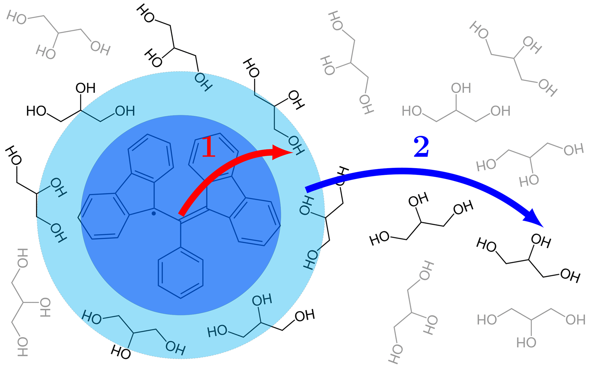
Figure 1Two conceptually different steps of the polarization transfer process in liquids. (1) Direct transfer from the electronic spin on the free radical to the proximate nuclear spins on the solvent molecules due to dipolar interaction. (2) Diffusion of the proximate solvent molecules to the bulk.
Given that every solvent molecule gets directly polarized and also spreads the polarization, the distinction between the two steps of polarization transfer in liquids (Fig. 1) is conceptual and does not reflect fundamental differences in the mechanisms of the two steps. In fact, both steps are enabled by molecular diffusion which sometimes brings a solvent molecule closer to the radical and sometimes takes it further away. Since the analytical description of translational diffusion in simple liquids is well developed (Ayant et al., 1975; Hwang and Freed, 1975), a unified theoretical treatment of the two steps of polarization transfer becomes possible, as we demonstrate in the present paper.
From the six terms of the dipolar alphabet, the part that contributes to the solid effect is (Wenckebach, 2016), where
Here is the dipolar constant, γS and γI are the gyromagnetic ratios of the electronic and nuclear spins, and are the spherical polar coordinates of the vector pointing from one of the spins to the other. The angular dependence of A1 is that of a second-degree spherical harmonic of order m=1, as implied by the subscript. The need for direct polarization of the solvent nuclei in liquids increases the shortest possible distance r in Eq. (1) and thus reduces the largest achievable dipolar coupling. This requirement for interaction across a larger distance, however, does not explain why the solid effect works in solids but is compromised in liquids.
To understand the difference between solids and liquids one should consider the time-correlation function of the dipolar interaction:
Here the inner angular brackets with the subscript t′ denote averaging with respect to the time point t′ along the random trajectory of a single nuclear spin. Because every nucleus encounters the electronic spins millions of times during its T1 relaxation time, this average should be the same for all nuclei in the liquid. Thus, in addition to the time averaging, in Eq. (2) we also average over the ensemble of identical nuclear spins in the sample (outer angular brackets).
Now, if the dipolar correlation function (Eq. 2) decays on timescales that are much longer than some relevant characteristic time, then the experiment essentially detects the initial value . The last ensemble average over all electron–nucleus pairs requires integration over the spatial variables and multiplication by the concentration N of the unpaired electrons:
(The factor comes from the normalization of the spherical harmonic .) This slow-motional limit corresponds to the situation in solids under the (unrealistic) assumption of fast and efficient spin diffusion. If, on the other hand, the decay time of the correlation function is much shorter than the relevant characteristic timescale, then the experiment detects the long-time limit . The solid effect vanishes because the average of the spherical harmonic over the angles gives 〈A1〉=0. This fast-motional limit corresponds to low-viscosity liquids in which the dipolar interaction is averaged out. To the extent that they exhibit the solid effect, viscous liquids must lie somewhere between these two extremes.
The interpolation between these two limiting cases on the basis of the dipolar correlation function is formally developed in Sect. 3. This task requires a time-domain description of the solid effect, similar to the treatment of relaxation by random motion where the correlation function arises from second-order, time-dependent perturbation theory (Abragam, 1961, chap. VIII). In principle, there are two such time-domain descriptions that we can utilize for the treatment of the solid effect in liquids. The first is the rate-equation formalism, which models the dynamics of the electronic and nuclear polarizations, and the second is the description developed in Sezer (2023a), which additionally accounts for the dynamics of the coherences. Both of these options will be explored in Sect. 3. When modeling the stochastic dynamics of the dipolar interaction, we resort to the stochastic Liouville equation (SLE) of Kubo (1954) and Anderson (1954), rather than to second-order perturbation theory. In agreement with previous work (Papon et al., 1968; Leblond et al., 1971a), our analysis shows that the characteristic timescale against which the dipolar correlation time should be compared is the electronic T2 relaxation time.
In the next two subsections we summarize the time-domain analysis of Sezer (2023a).
2.2 Rate equations
The dynamics of the electronic polarization, PS, is justifiably taken to be independent of the dipolar interaction with the nuclear spins, as other mechanisms relax the electrons more efficiently. With R1S denoting the rate of electronic T1 relaxation, and v1 the rate constant of the mw excitation of the (allowed) EPR transition, the rate equation of the electronic polarization is
Here is the equilibrium (Boltzmann) electronic polarization and the dot over the symbol denotes differentiation with respect to time. Solving this equation for at steady state, we arrive at the ratio
where s is the familiar electronic saturation factor. We refer to p as the electronic polarization factor, since p=0 indicates that the steady-state polarization has vanished, and p=1 indicates that it is identical to the Boltzmann polarization (i.e., maximally polarized).
The rate equation of the nuclear polarization, PI, is
where R1I is the nuclear T1 relaxation rate, and the phenomenological rate constants v± quantify the mw excitation of the forbidden transitions. The steady state of Eq. (6) is
where was used in the last term.
As the derivations in Sect. 3 consider only the effect of mw excitation, we have written Eq. (7) such that the relaxation contribution is on the left and the mw contribution on the right of the equality. Subsequently, to identify the phenomenological rate constants v±, we will match the terms on the right-hand side with the predictions of the proper analysis in liquids.
From Eq. (7) we find the DNP enhancement
where the first equality is the definition of ϵ and
From ϵSE it is clear that the solid effect benefits from large pv− and small . The ratio pX in Eq. (9) is analogous to the electronic polarization factor Eq. (5), and we call it the nuclear cross-polarization factor. In liquids, v+ is typically negligible compared to the nuclear spin-lattice relaxation rate, and pX≈1. Then,
2.3 Spin dynamics
The dynamics of the quantum-mechanical expectation values sn of the electronic spin operators Sn () is described by the classical Bloch equations
The matrix in Eq. (11) contains the electronic transverse relaxation rate R2S, the mw nutation frequency ω1 and the offset between the electronic Larmor frequency ωS and the mw frequency ω.
In Sezer (2023a) we visualized such coupled differential equations diagrammatically. In our visual depiction, the time derivative of a dynamical variable, like sn, is represented by an oval node. The contributions to this time derivative, which are on the right-hand side of the differential equation, are represented by arrows that flow into that node (Fig. 2a). The contribution of a given arrow is obtained by multiplying the weight of the arrow by the variable from which the arrow originates. The self-arrows that exit from an oval node and enter the same node correspond to the relaxation terms along the diagonal of the Bloch matrix. The negative sign of the weight of a self-arrow is written separately inside the loop formed by the arrow. The constant variable in the inhomogeneous term of the Bloch equations (Eq. 11) is represented by a gray rectangular node. With this notation, the Bloch equations are depicted by the four nodes in the top row of Fig. 2a and by the black arrows connecting these nodes.
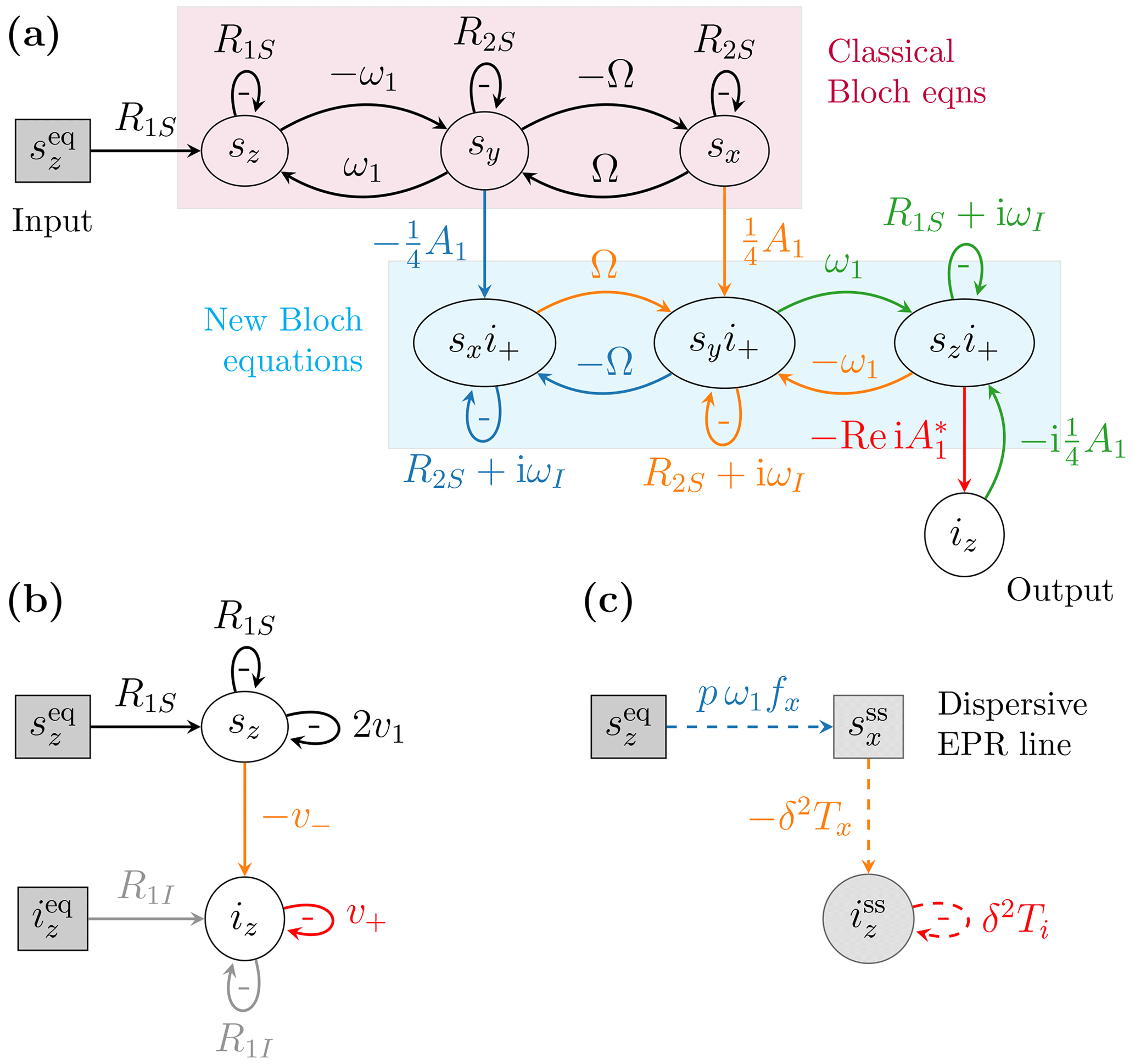
Figure 2Diagrammatic representation of (a) the equations of motion of the spin dynamics relevant to the solid effect, namely Eq. (11) (purple rectangle), Eq. (12) (cyan rectangle) and Eq. (14), and (b) the rate equations of the electronic and nuclear polarizations (Eqs. 4 and 6). (c) Steady-state relationships between the input and output variables.
The lower half of Fig. 2a shows the dynamics of the electron–nuclear coherences that are relevant for the solid effect. In particular, the quantum-mechanical expectation values of the operators SnI+ (), which we denote interchangeably by gn and sni+, evolve according to the following coupled differential equations (Sezer, 2023a):
where
The matrix 𝔅 is essentially the Bloch matrix but with the nuclear Larmor frequency ωI added as an imaginary part to its main diagonal. The time derivatives of gn in Eq. (12) are represented by the three oval nodes enclosed in the cyan rectangle in Fig. 2a. The arrows between these nodes are seen to exactly replicate the classical Bloch equations in the rectangle above them. The inhomogeneous term in Eq. (12) couples the dynamics of the variables gn to the transverse components of the electronic magnetization, on the one hand, and to the longitudinal component of the nuclear magnetization, on the other. All these couplings scale with the dipolar interaction A1. They play an essential role in the solid effect, as they connect the Boltzmann electronic polarization to the nuclear polarization (labeled “Input” and “Output” in Fig. 2a).
Lastly, the coherent dynamics of the operator Iz, whose expectation value is denoted by iz, is
where Re takes the real part of a complex number. In Fig. 2a this equation is represented by the oval node iz (labeled “Output”) and the red arrow flowing into it.
In liquids, the weights A1 fluctuate randomly due to molecular diffusion. When extending the formalism to liquids (Sect. 3.3), we will transform Eq. (12), which constitutes a system of coupled differential equations, to an SLE (Kubo, 1969) that describes the spin dynamics under random modulation of A1.
For comparison, Fig. 2b shows the dynamics of the longitudinal components implied by the rate equations (Eqs. 4 and 6). Visual inspection of Fig. 2a and b makes it clear that the rate constant v− provides a reduced description of the complicated network connecting sz to iz. Similarly, the rate constant v+ accounts for the self-influence of iz mediated by the coherences in the second set of Bloch equations (enclosed in the cyan rectangle). In (Sezer, 2023a), we identified the rates v± and v1 by requiring that the dynamics in Fig. 2a and b reached identical steady states.
At steady state, the three dynamical variables of the classical Bloch equations (Eq. 11) were related to each other and to the electronic Boltzmann polarization as follows:
where
(Comparing the last equality in Eq. (15) with Eq. (5) we found that p=R1Sfz and that the rate constant of the allowed EPR transition was .)
Solving the second set of Bloch equations (Eq. 12) at steady state, and substituting in Eq. (14), we obtain
where the dipolar interaction is isolated in
Since the transverse components are related to the Boltzmann polarization (Eq. 15), the right-hand side of Eq. (17) is of the form
where
(The superscript “T” indicates transpose, and is the ijth element of the inverse matrix 𝔅−1.) Because 𝔅 has units of inverse time, Ti and Ts have units of time.
We note that Ts receives contributions from both and . As was shown in Sezer (2023a), it is possible to rewrite the contribution of the former as if it also came from . In other words, the entire contribution of to the derivative of iz at steady state can be expressed as if it is mediated only through the dispersive component , as depicted in Fig. 2c. (Dashed arrows represent mathematical relationships between the variables that hold at steady state. Differently from the solid arrows, which correspond to causal dependencies governing the dynamics at all times, the dashed arrows need not reflect direct causal dependence. A rectangular node indicates that the inflowing arrows contribute directly to the value of the variable and not to its time derivative. The gray shade of the nodes signals that the variables remain constant in time, as they should at steady state.)
In addition to , in Eq. (20) we also need and . These are , and , where the functions
play an analogous role in the steady-state analysis of the second set of Bloch equations as the functions fy, fx and fz (Eq. 16) in the classical Bloch equations. In terms of these,
where
(The functions in Eq. 23 emerge from lumping the contribution of to that of , as mentioned above.)
With Ti and Ts determined, the forbidden-transition rates on the right-hand side of Eq. (7) become
where the mw-independent part of Ti, namely
is subtracted in the first equality of Eq. (24) because it contributes to the nuclear T1 relaxation rate. (In Fig. 2a this mw-independent part corresponds to the loop formed by the green arrow from iz to gz and the red arrow in the opposite direction.)
2.4 The solid effect
Using the rate constants in Eq. (24), we rewrite the solid-effect DNP enhancement (Eq. 9) as
The functions pω1fx, Tx and in this expression are visualized in, respectively, the first, second and third rows of Fig. 3. The product of the first two rows, which appears in the numerator of Eq. (26), is shown in the fourth row of the figure. In the right margin of the figure, we have included the flow diagram from Fig. 2c, which has been straightened here so that the weights of the arrows correspond to the respective rows. Note that the dipolar interaction strength, δ, and the nuclear spin-lattice relaxation rate were not needed to calculate the properties in the first four rows of the figure. (They will be needed for the last two rows.)
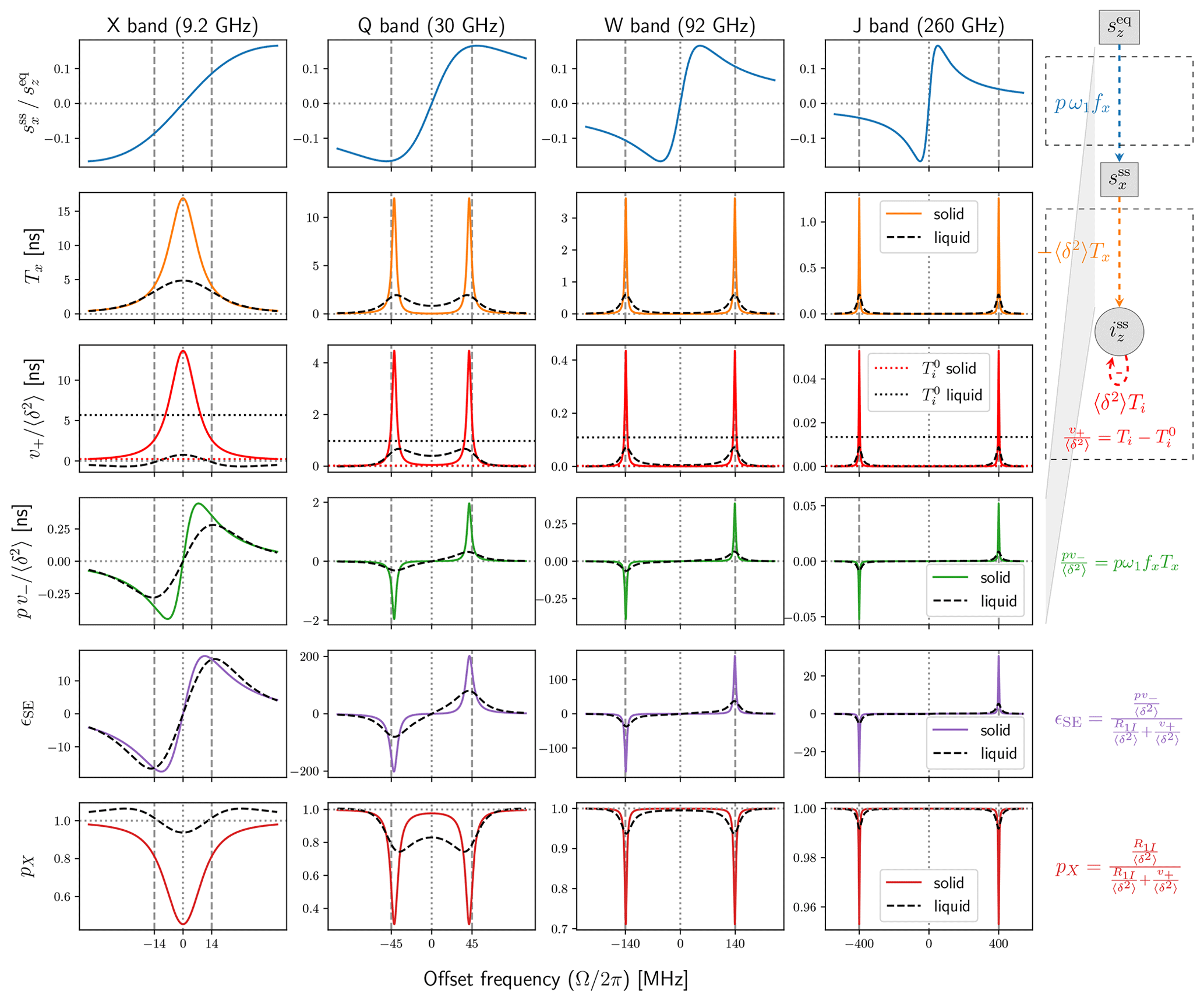
Figure 3Comparison between solids (with fast spin diffusion) and liquids. First row: dispersive component of the power-broadened EPR line. Second and third rows: relevant transfer functions of the new Bloch equations in Fig. 2a. Fourth row: the product of the first and second rows, which relates the input to the output . Fifth row: DNP enhancement calculated from the third and fourth rows using . Sixth row: nuclear cross-polarization factor calculated from the third row using . Simulation parameters: T2S=60 ns, T1S=9 T2S, B1=6 G (converted to ω1 assuming g=2), contact distance b=1 nm, radical concentration N=0.1 M, and T1I of 4.7 ms (X band), 27.4 ms (Q band) and 50 ms (W and J bands). The dipolar correlation time of the liquid simulation (dashed black lines) is ns.
While different magnetic fields B0 yield different relaxation times, for illustrative purposes we used the same electronic T1 and T2 times for X, Q, W and J bands. We additionally used the same mw field (B1=6 G) at all bands. Hence, the steady state of the classical Bloch equations (Fig. 3, first row) is identical across the four columns of the figure. The solid blue lines, which correspond to the dispersive component of the power-broadened EPR line, are identical but appear different due to the different scalings of the horizontal axes. The absorptive component is much smaller under the power-broadening conditions considered here and is not shown. However, its contribution is exactly accounted for in the analysis. (This was the reason for introducing the functions in Eq. 23.) Anticipating the liquid state, we observe that the classical Bloch equations are independent of the dipolar coupling A1 (Fig. 2a). Hence, the first row of Fig. 3 will not change when going to liquids because we use identical relaxation rates.
The transfer functions Tx and encapsulate all relevant steady-state properties of the second set of Bloch equations, as well as their coupling to the classical Bloch equations and to iz through the dipolar interaction (Fig. 2a). These functions are visualized in the second and third rows of Fig. 3 (orange and red lines). The solid colored lines are calculated using the equations given above and correspond to solids, subject to the (unrealistic) assumption of very fast spin diffusion. The dashed black lines are calculated as described in the next section and correspond to liquids. Clearly, the time-dependent modulation of the dipolar interaction in liquids has a dramatic effect on these functions.
The fourth row in Fig. 3 shows the product of the blue lines in the first row and the orange lines in the second row and corresponds to the total transfer function from the primary input, , to the ultimate output, iz (Fig. 2a). With the exception of X band, going from solids to liquids substantially reduces the peaks of pv−. (We used identical relaxation parameters for liquids and solids to highlight the role of the dipolar correlation time.)
The transfer functions in the first four rows of Fig. 3 depend only on the electronic relaxation times (assuming ). To calculate the enhancement ϵSE and the nuclear cross-polarization factor, pX, which are shown in the last two rows of Fig. 3, we had to select specific values for R1I and δ2. For the latter, we used the ensemble-averaged static value from Eq. (3),
which applies to solids with fast and efficient spin diffusion. The numerical calculations in Fig. 3 are for contact distance bref=1 nm and radical concentration Nref=0.1 M. These are realistic but otherwise arbitrary values.
For the purposes of illustration we wanted to use the same R1I for all four mw bands in the figure. In this way, by comparing the four columns with each other, one would be able to assess the effect of changing only B0. This strategy worked for solids, at least for the numerical values that were used, but failed for liquids due to the very different contributions of Ti to the nuclear relaxation rate (denoted by in Eq. 25). This part of Ti is shown in the third row of Fig. 3 with horizontal dotted lines. The dotted red lines for solids are very close to zero. The more visible dotted black lines for liquids change dramatically with the mw band. Since the total relaxation rate R1I must be larger than the contribution of , the nuclear T1 had to be only a few ms at X band. Using such small T1 at J band, however, gave tiny liquid-state DNP enhancements.
Even if, admittedly, our calculated enhancements are only illustrative, in an effort to have somewhat realistic nuclear T1 relaxation times, we used T1I=50 ms when the corresponding rate R1I was larger than and used otherwise. This resulted in the following nuclear T1 relaxation times: 4.7 ms (X band), 27.4 ms (Q band) and 50 ms (W and J bands). These were used for both liquids and solids. Naturally, the choice of different nuclear T1 times has a direct influence on the calculated enhancements. For example, the peak DNP enhancements at X and W bands differ by about 1 order of magnitude (purple lines in the fifth row of Fig. 3) mostly because the nuclear T1 times at these two bands also differ by 1 order of magnitude.
The theory behind the liquid calculations in Fig. 3 is presented in the next section.
3.1 Molecular motion as a random process
Let us denote the components of the inter-spin vector collectively by ζ. To describe the solid effect in liquids we consider a random process that changes ζ and thus modulates the dipolar interaction between the two types of spins.
When the random dynamics of ζ is modeled as a discrete-state process, the probabilities of observing the different discrete states are collected in the vector p(t). This probability vector evolves in time as , where the matrix K contains the rate constants of the random transitions between the states. All eigenvalues of such stochastic matrices are non-negative, and, for an ergodic chain of states, only one of the eigenvalues equals zero. In general, the stochastic matrix K is not symmetric, which means that there are a right eigenvector and a left eigenvector associated with each eigenvalue. The right eigenvector of the zero eigenvalue corresponds to the vector of equilibrium probabilities, peq, and the left eigenvector of the zero eigenvalue corresponds to the vector 1, which contains ones in all of its entries. Note that 1Tpeq=1.
When the random dynamics of ζ is modeled as a continuous-state diffusion process, then the time evolution of the probability density p(ζ,t) is described by a Fokker–Planck equation of the form
where Kζ is a linear differential operator acting on the ζ dependence of p(ζ,t). As in the discrete case, the eigenvalues of Kζ would be non-negative, and one eigenvalue would equal zero. The corresponding right eigenfunction is the equilibrium probability density peq(ζ), and the left eigenfunction is constant in ζ.
For brevity, we will also adopt the discrete notation for the continuous case. In particular, we will use italic bold symbols to indicate the dependence on ζ and will denote operators that act on the ζ dependence with non-italicized capital bold symbols. With this understanding,
will apply to both the continuous and discrete cases. Similarly, 1Tf will imply integration over the ζ dependence of the function f(ζ) in the continuous case and summation over all different states in the discrete case.
Note that in the probabilistic description of the random process by the Fokker–Planck equation (Eq. 28), the probability density p(ζ,t) characterizes an ensemble of nuclei, and ζ is treated as an independent variable which is not a function of t. In contrast, when a single nucleus is followed in time (e.g., through molecular dynamics simulations), ζ is a random function of t. Although this second picture of random trajectories was invoked when writing the dipolar correlation function in Eq. (2), in the following pages we only work with the probabilistic description of an ensemble of identical nuclei.
Below, we will use the dynamical rule (Eq. 29) when combining the stochastic dynamics of ζ with the spin dynamics from Sect. 2. The combined dynamics will be described by a stochastic Liouville equation (SLE) for a ζ-conditioned spin variable. In the case of the nuclear polarization, for example, the SLE will describe the dynamics of PI(t), which stands for PI(ζ,t) in the continuous case. For a detailed explanation of SLE the reader is referred to the literature (Kubo, 1969; Gamliel and Levanon, 1995). A more recent discussion can be found in Kuprov (2016).
3.2 Rate equations in liquids
3.2.1 Electronic polarization
The electronic polarization was assumed to be insensitive to the dipolar coupling with the nuclear spins. Hence, the ζ-conditioned electronic polarization PS(t) is of the following separable form:
in which all ζ dependence is isolated in the equilibrium probability of the stochastic process. From PS(t) we obtain the averaged (over ζ) electronic polarization by summing/integrating over the ζ dependence. This is done with the help of the constant vector/function 1 as follows:
(In the last equality we used the normalization of the probability, 1Tpeq=1, which reads in the continuous case.) Note that PS(t) in Eq. (30) is, in fact, the electronic polarization averaged over the stochastic variable (Eq. 31).
In this description, the experimentally accessible polarizations correspond to the averaged values, while the ζ-dependent variables, like PS(t), serve only an intermediate, book-keeping role. In other words, at the end we will always average over ζ by using the constant vector/function 1.
Since Eq. (30) holds in general for the electronic polarization, it also holds at steady state and at equilibrium:
Here and are the averaged (over ζ) values which correspond to the macroscopic polarization.
Lastly, we point out that at equilibrium all joint spin-ζ properties are of the above separable form. In other words, the last equality in Eq. (32) is not limited to the electronic polarization but applies to all other equilibrium properties.
3.2.2 Nuclear polarization
To illustrate the SLE formalism and to introduce further notation, we start by transforming the rate equation of the nuclear polarization (Eq. 6) to an SLE:
There are several different things going on here, so let us examine them one by one.
First, following the convention introduced above, PI(t) stands for PI(ζ,t), which is the nuclear polarization conditional on the random state ζ. In this case the dot indicates partial derivative with respect to the time dependence, at fixed ζ. Second, the term KPI drives the dynamics in the ζ space by providing “off-diagonal” elements that mix the different random states. All remaining terms on the right-hand side of the SLE are “diagonal” in the ζ space and act only on the spin degree(s) of freedom (which are conditioned on ζ). Third, the mw excitation rates v± and the relaxation rate R1I have acquired ζ dependence, turning into operators in ζ space that act on PI(t) or peq. In the discrete case, these would be matrices with different v± and R1I values for each discrete state ζ along their main diagonals. We use hollow capital letters to denote such “diagonal” operators in ζ space, also in the continuous case. Fourth, as all equilibrium properties, the nuclear Boltzmann polarization is separable, with the ζ dependence confined to the equilibrium probability of the random process.
The steady state of Eq. (33) is
where we used (Eq. 5). Our aim is to solve Eq. (34) for and then obtain the macroscopic nuclear polarization by calculating the average .
Clearly, solving Eq. (34) consists of calculating the inverse of the operator . This is a daunting task in general and requires the matrix representation of K in some basis set. Here we will limit the discussion to random motions that are orders of magnitude faster than the nuclear T1 relaxation rate, which we concluded to be the case even in viscous liquids like glycerol. This assumption ensures that, at steady state, all nuclear spins in the sample are equivalent and have the same polarization. Hence, we will look for a separable steady-state solution of the form
With this ansatz, Eq. (34) becomes
While the difference between Eqs. (34) and (36) appears to be minor, in fact we have achieved a tremendous simplification since Kpeq=0, and thus the dynamical aspect of the random process is gone; only its equilibrium (i.e., time-independent) properties remain. Indeed, since in Eq. (36) all ζ operators act on the equilibrium probability peq, integration over the ζ dependence brings the average values:
(These are the average values of the ζ-dependent functions R1I(ζ) and v±(ζ), respectively.) After averaging, Eq. (36) becomes
Comparison of Eqs. (38) and (7) shows that the phenomenological rates R1I and v± in the rate equation should be identified with the macroscopic averages 〈R1I〉 and 〈𝕍±〉 over the liquid sample. This is the familiar regime of fast motion, where one observes the averaged values of the magnetic parameters. We have thus provided a formal justification of why the averaged δ2 in Eq. (27) corresponds to fast spin diffusion in the case of solids.
We observe that the static averages over 3D space, which are implied by Eq. (37), do not allow for the partial dynamical averaging of the dipolar interaction. As discussed above, such averaging should be based on the time-correlation function of A1. However the rate constants v± always contain the square of the dipolar interaction and do not provide access to A1 itself. We thus conclude that the partial averaging of the dipolar interaction in liquids is inaccessible to modeling by rate equations.
3.3 Spin dynamics in liquids
To gain access to the dipolar interaction before it is squared, we turn to the equations of motion of the coherences from Sect. 2.3. We first transform the equation of iz (Eq. 14) to an SLE:
As before, iz(t) and gz(t) stand for iz(ζ,t) and gz(ζ,t) in the continuous case, K acts on the ζ dependence of iz and has become a “diagonal” operator in ζ space. Averaging Eq. (39) over ζ, we obtain the macroscopic equation
At steady state, using the ansatz for liquids (Eq. 35) in the form , we have
Since we accounted only for the coherent contribution to the time derivative of iz, the right-hand side of Eq. (41) corresponds to the right-hand side of Eq. (7). Our aim is to identify the phenomenological rate constants v± that should be used in Eq. (7) by analyzing . However, because the random modulation of A1 additionally contributes to the nuclear T1 relaxation, we have the equality
from which we will read out the desired rates.
3.3.1 Contribution to nuclear T1 relaxation
The contribution of to the nuclear spin-lattice relaxation can be identified by its value in the absence of mw irradiation. From Eqs. (12) and (13) we see that for ω1=0 the dynamics of gz completely decouples from gx and gy. The SLE of gz in this case becomes
Technically, R1S and ωI should be operators that act on the ζ dependence of gz. However, we take the electronic T1 relaxation rate and the nuclear Larmor frequency to be independent of the dipolar coupling, which is parametrized by ζ. The corresponding operators are then R1S𝕀 and ωI𝕀, where 𝕀 is the identity operator in ζ space. This identity operator will not be written explicitly.
The steady-state solution of Eq. (43) is
where we again used the ansatz for liquids. Substituting this on the left-hand side of Eq. (42), we find that the nuclear relaxation rate due to A1 is
To express this relaxation rate in a more intelligible manner, we observe that the inverse of a matrix M whose eigenvalues have strictly positive real parts can be written as
Applying this identity to the matrix in Eq. (45), we find
where
is the time-correlation function of the dipolar interaction (Eq. 2). Since the integral in Eq. (47) corresponds to the Laplace transform
we have
The real part of the Laplace transform is known as spectral density. Here the spectral density is evaluated at a the complex argument R1S+iωI, which contains both the nuclear Larmor frequency and the electronic T1 relaxation rate.
Let us examine Eq. (50) in the solid-state limit where A1 does not change with time. Then and
In Abragam's nomenclature (Abragam, 1961) this is relaxation of the second kind, meaning that it is due to the relaxation of the electronic spins and not due to the modulation of the dipolar interaction by motion. This was shown with horizontal, dotted red lines in the third row of Fig. 3.
In the case of liquids, we expect C11(t) to decay with time. Assuming a mono-exponential decay with correlation time τ,
This was shown with horizontal, dotted black lines in the third row of Fig. 3. To understand why it increases with decreasing ωI, let us examine the case of motion that is faster than the electronic T1 time, i.e., . The result,
is relaxation of the first kind with Lorentzian spectral density. Clearly, smaller ωI implies larger dipolar contribution to the nuclear T1 relaxation rate.
Having identified the relaxation rate on the right-hand side of Eq. (42), we now proceed with the analysis of the rates v± characterizing the forbidden transitions.
3.3.2 Contribution to forbidden transitions
Combining the dynamics of the coherences (Eq. 12) with the stochastic dynamics (Eq. 29), we arrive at the following SLE:
Note that the matrix 𝔅 does not depend on time as the electronic relaxation properties were taken to be insensitive to the dipolar interaction between the electronic and nuclear spins. Recall that the operators written as upright bold letters (including the hollow ones) act on the ζ dependence of the variables, which is encoded by the italic bold symbols. The script uppercase letters denote 3×3 matrices, which act on the column vectors that are shown explicitly.
Although not shown explicitly in Eq. (54), we imply the tensor products of the operators K, 𝔅 and 𝔸1 with the identity operators in the spaces on which K, 𝔅 and 𝔸1 do not act (i.e., K and 𝔸1 are in fact ℐ⊗K and ℐ⊗𝔸1 where ℐ is the 3×3 identity matrix, and 𝔅 is 𝔅⊗𝕀 where 𝕀 is the identity operator in the ζ space).
Before solving Eq. (54) at steady state, let us introduce the (right) eigenvalue problem of 𝔅,
where the diagonal matrix
contains the eigenvalues of 𝔅 along its main diagonal, and the columns of the 3×3 matrix 𝔘 contain the corresponding right eigenvectors. Then, the steady state of Eq. (54) is
which, after inverting the matrices, yields
Plugging this solution for into the left-hand side of Eq. (42), and defining the matrix
we find
Comparison with the right-hand side of Eq. (42) yields
where we used the relationships between and (Eq. 15) to arrive at v−.
We observe that ℒ is a 3×3 diagonal matrix without any ζ dependence since the right-hand side of Eq. (59) is averaged over ζ. With , we have
Using Eq. (46), these diagonal elements can be written as
where we used Eq. (48) in the third equality and Eq. (49) in the last one. Hence, each Ln is the Laplace transform of the time-correlation function C11(t) evaluated at the eigenvalue λn of 𝔅. The matrix ℒ to be used in Eq. (61) is thus
In summary, for any given set of parameters, we form the 3×3 matrix 𝔅 (Eq. 13) and numerically calculate its eigenvalues and right eigenvectors. The former are used in Eq. (64) to calculate ℒ. Sandwiching ℒ by the eigenvectors, as required in Eq. (61), we arrive at the desired rates v±. This prescription applies to any motional model describing the stochastic dynamics of the inter-spin vector. Different models will differ only in their spectral densities J11.
From a mathematical point of view, the simplest case is a model with exponential dipolar correlation function, , where τ is the correlation time. Then
and Eq. (64) becomes
All dashed black lines labeled “liquid” in Fig. 3 were calculated using Eq. (66) with τ=12 ns.
Comparing v+ and pv− (Fig. 3, third and fourth rows) between the solid and liquid cases, we see that at Q, W and J bands, the fluctuations of the dipolar interaction have substantially broadened the lines centered at the canonical solid-effect offsets and have reduced the peak enhancements in liquids compared to solids (fifth row). At X band, where the two lines had already merged in the solid case, the effect of fluctuations is qualitatively different, although line broadening is also visible. Most strikingly, the rate v+ is seen to become negative at offsets larger than ωI, which leads to a nuclear polarization factor (Eq. 9) that exceeds 1 (Fig. 3, bottom row).
4.1 Translational diffusion of hard spheres
A mono-exponential dipolar correlation function is a poor model of translational diffusion in liquids. The so-called force-free hard-sphere (FFHS) model, which assumes spherical molecules that contain the spins at their centers, is a more realistic yet analytically tractable model (Ayant et al., 1975; Hwang and Freed, 1975). It is universally employed in the analysis of diverse magnetic-resonance measurements, including nuclear relaxation by paramagnetic impurities (Okuno et al., 2022) and DNP via the Overhauser effect (Franck et al., 2013).
Because the spins are taken to be at the centers of the spherical molecules, the FFHS model has only two parameters: the coefficient of translational diffusion, D, and the distance of the spins upon contact of the spherical molecules, b. These two parameters form the characteristic motional timescale of the model (Ayant et al., 1975):
The Laplace transform of the dipolar correlation function of this model is (Ayant et al., 1975, Eqs. 51 and 55)
Using in Eq. (64) we calculated numerically the same properties as in Fig. 3 but for the FFHS model. The results are shown with colored solid lines in Fig. 4. For comparison, the model with mono-exponential correlation function from Fig. 3 is also reproduced in Fig. 4 with dashed black lines.
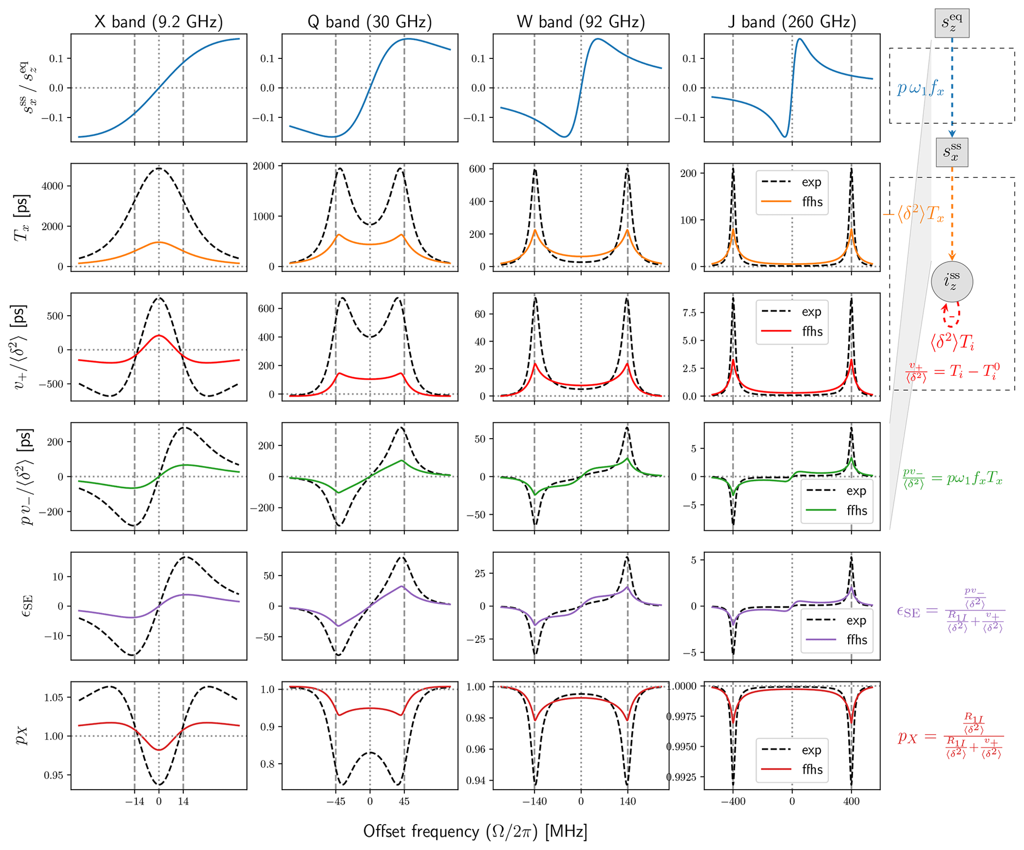
Figure 4Same as Fig. 3 for the model with exponential time-correlation function (dashed black lines) and the FFHS model (colored solid lines) both with ns.
The general observation from Fig. 3 that the fluctuation of the dipolar interaction broadens the solid-effect lines at is even more relevant for the FFHS model. Indeed, for the same dipolar timescale τ, the FFHS lines are much broader and, correspondingly, much smaller in peak amplitude than the lines of the exponential model. Hence, the FFHS model predicts significantly smaller DNP enhancements (Fig. 4, second last row) compared to the exponential model with the same timescale τ. At X band, the negative values of v+ are still present, but their magnitude is substantially reduced (third row). The corresponding offsets where the nuclear polarization factor, pX, is larger than 1 are similar in the two models, but again the deviation from 1 is much smaller in the FFHS model (last row).
Overall, pX in liquids is very close to 1 (last row of Fig. 4, FFHS model), which indicates that v+ is very small compared to R1I. In such cases, the solid-effect DNP enhancement (Eq. 9) is well approximated by Eq. (10). This explains why the enhancement in the fifth row of Fig. 4 is essentially a rescaled version of the row directly above it.
The substantial reduction of the peak intensities at the solid-effect offsets is accompanied by a smaller but still appreciable increase of the intensities at small offsets (Ω≈0). This trend is visible both in the transition from the solid case to a mono-exponential correlation function (Fig. 3, second row) and in the further transition to the FFHS model (Fig. 4). The significance of this observation will become clear in Sect. 4.4, where we compare our calculations with the experiments of Kuzhelev et al. (2022).
4.2 Approximate matrix inversion
Since 𝔅 is a 3×3 matrix, its eigenvalues and eigenvectors are easily determined numerically, as we did when calculating the exponential and FFHS models in Fig. 4. Nevertheless, to gain insight into the eigenvalue problem that is being solved, here we analyze Eq. (55) using perturbation theory. The analysis reveals that the eigenvalue problem is related to the effective magnetic field and the associated “tilted” coordinate frame (Wenckebach, 2016).
Let us introduce the matrix
where R1S in the lower right corner of 𝔅 (Eq. 13) has been replaced by R2S. The three eigenvalues of 𝔅0 are
where the frequency
corresponds to the effective magnetic field in the rotating frame. This field is tilted away from the z axis by an angle α such that
With the sine and cosine of α abbreviated as s and c, the right eigenvectors of 𝔅0 are
where the first column corresponds to λ0,0, the second to , and the third to . By inspection, , where the superscript “H” denotes Hermitian conjugation.
We treat the difference 𝔅−𝔅0 as a perturbation to 𝔅0. To first order in the perturbation, the eigenvalues of the original matrix 𝔅 are , where u0,n is the nth column of 𝔘0. Using this expression we find the corrected eigenvalues
with
Collecting the eigenvalues (Eq. 74) in the diagonal matrix , we have . As an example, the element in the lower right corner of the inverse matrix is
(This approximation of Fz was used in Sezer (2023a) without proof.)
From Eq. (76), and using the first equality in Eq. (22), we immediately find
To obtain v+, we need to subtract from Ti (Eq. 24). Since ω1=0 implies s=0 and c=1,
which is identical to the exact result in Eq. (25). Hence,
One can similarly obtain the rate constant v− as a linear combination of the reciprocals of the approximate eigenvalues and . The result is
with
Recall that (Eq. 24).
The first eigenvalue in Eq. (74) does not depend on the offset Ω. The other two eigenvalues depend on the offset through ωeff. Let us consider sufficiently large offsets such that , and so . This condition is satisfied at the solid-effect offset positions at W and J bands but may be entirely inapplicable to X band at large mw powers, as discussed in Sezer (2023a). When the condition holds, s≈0 and c≈1, and the eigenvalues in Eq. (74) become and . Thus correspond to complex-valued Lorentzians centered at and with widths equal to the homogeneous EPR line width (without power broadening). These are the Lorentzians that we see as narrow lines at W and J bands in the second and third rows of Fig. 3 (orange and red solid lines).
In the case of motion, assuming mono-exponential correlation function for simplicity, each eigenvalue is replaced by . This amounts to increasing the widths of the solid-effect Lorentzians from R2S to . The resulting motional broadening is the reason for the differences between the “solid” and “liquid” lines in the second and third rows of Fig. 3.
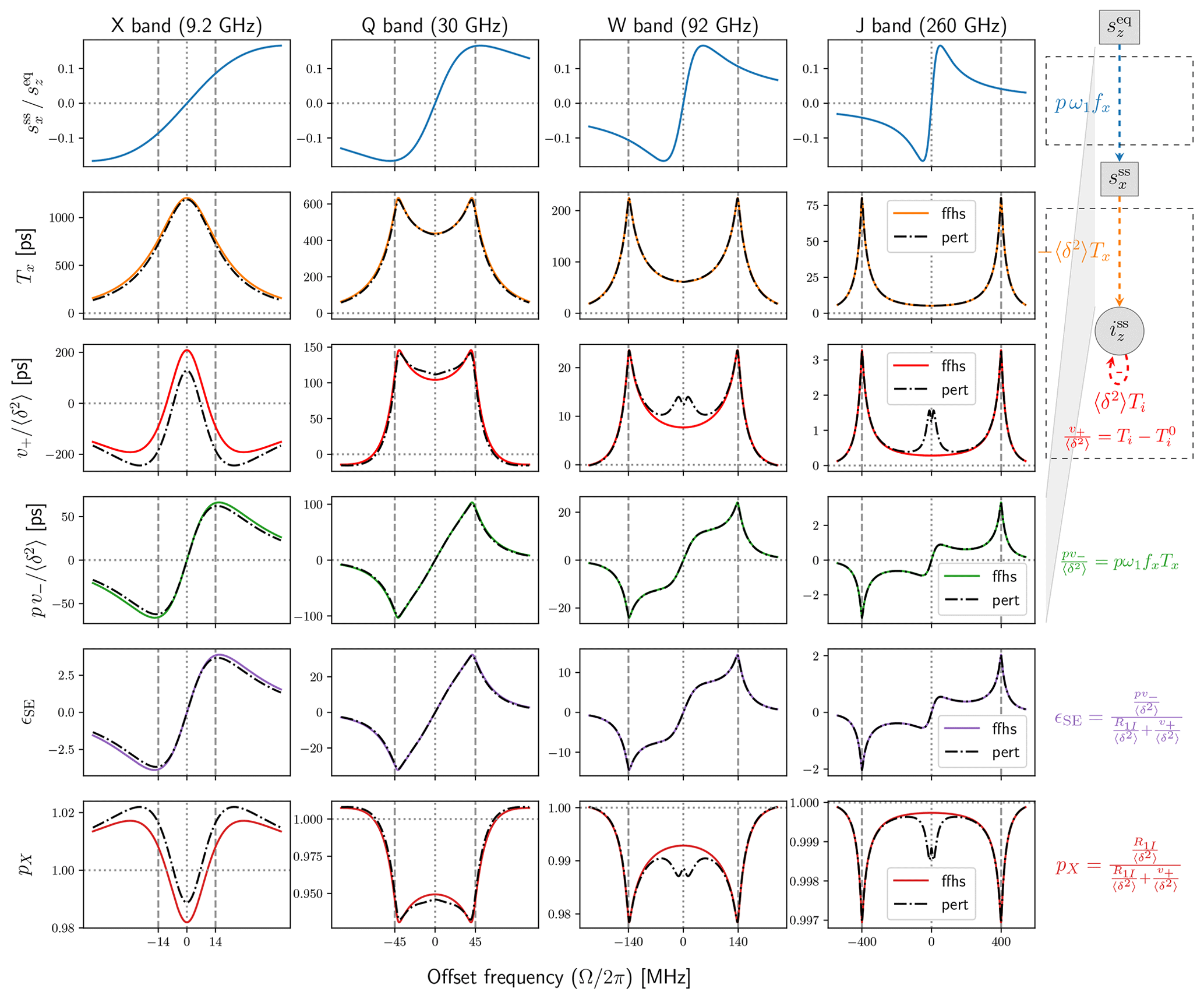
Figure 5Comparison between the exact (solid colored lines) and perturbative (dashed black lines) calculations of the FFHS model. All parameters as in Fig. 4. The eigenvalue problem of the generalized Bloch matrix 𝔅 has a simple closed-form solution when T1S=T2S. The perturbative approximation uses these analytical eigenvectors and corrects the eigenvalues to first order in the difference .
For a general motional model, we have the approximate , which yields the approximation to be used in Eq. (61). For the spectral density of the FFHS model, the perturbative expressions are compared with the exact numerical calculation in Fig. 5. The former are plotted with dashed–dotted black lines and the latter with colored solid lines, like in Fig. 4. We see that the perturbative analysis is satisfactory in general, at least for the specific choice of parameters that were used. It gives excellent predictions for v− (Fig. 5, fourth row) and, because the two are related by a global scaling factor (Eq. 10), also for the DNP enhancement (fifth row). At the same time, it is seen to consistently fail for the rate v+ at small offsets in the vicinity of the origin (third row).
We should mention that the perturbative approximation becomes progressively better when R2S approaches R1S (not shown), as it is exact for R2S=R1S.
Leaving the approximation quality of the perturbative analysis aside, we observe that the enhancement profiles in the fifth row of Fig. 5 reveal the emergence of a novel feature at small offsets. At W band, this feature appears as a shoulder in the broadened lines, and at J band it is already separated from the canonical solid-effect peaks. Comparison with the lines in the first row of Fig. 5 makes it clear that this new feature in the DNP spectrum coincides with the extrema of the dispersive component of the power-broadened EPR line. For saturating mw powers, where ω1≫R1SR2S, these extrema are at
(The subscript was selected because these are also the offset positions where the electronic saturation factor equals one half.) The factor pv− in the fourth row of Fig. 5 is obtained as the product of the first and second rows, as elaborated in Sezer (2023a). When the solid-effect lines at (second row) become sufficiently broad, their amplitude at gets large enough for the peak of the dispersive EPR line (first row) to be visible in the DNP spectrum.
4.3 Motional suppression and broadening
Let us examine more closely the suppression of the lines at the solid-effect offsets and the concurrent increase of their intensity at . We will limit the discussion to J band where the condition ωI≫ω1 holds, and the solid-effect offsets are . Using the perturbative eigenvalues in Eq. (74), we see that only the real parts of survive at these offsets. The peak amplitudes of the solid-effect lines are then proportional to J11(R2S).
The limits τ≪T2S and τ≫T2S correspond to, respectively, very fast and very slow diffusive motion relative to the electronic T2. In the slow limit τ≫T2S, we have
for both the mono-exponential and FFHS motional models. This means that, in solids, the peaks increase with the electronic T2. In the opposite limit of very fast motion, i.e., τ≪T2S, we find
which means that, in liquids, the peak amplitudes are proportional to the dipolar correlation time τ. In other words, faster fluid diffusion (i.e., smaller τ) corresponds to smaller peaks and thus smaller solid-effect enhancement at the canonical offsets. We also see that for the same τ the peaks of the FFHS model are less than half of the peaks of the exponential model, which is in agreement with Fig. 4 (second and third rows).
To describe the transition between the fast and slow limits, we define the reduction factor
which equals one in the solid limit and approaches zero for small τ. Since it quantifies how much smaller the peaks are compared to the solid case, ρ is a measure of how “solid-like” the liquid is.
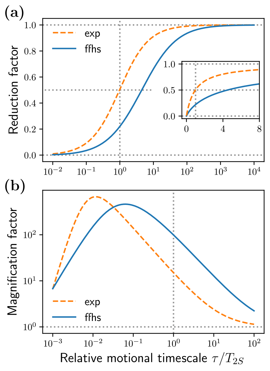
Figure 6Multiplicative deviation of Tx(Ω) from the solid limit at (a) the solid-effect offsets and (b) the offsets for the exponential and FFHS models.
Figure 6a shows the reduction factors of the exponential and FFHS models against the relative motional timescale . For the exponential model, the solid-effect peaks drop to half of their maximum values at τ=T2S. In the case of the FFHS model, this happens already at τ≈4T2S (see inset). In other words, appreciable reduction compared to the solid limit occurs even for exceedingly long diffusive timescales, several-fold compared to the electronic T2. For identical τ's the exponential model is seen to be more solid-like than the diffusive FFHS model across the entire motional range. Hence, realistic translational diffusion suppresses the solid-effect peaks more effectively than mono-exponential decay.
As a quantitative measure of the motional broadening, let us consider the magnitude of Tx (Fig. 5, second row) at the locations of the extrema of the dispersive EPR line (first row). Since the intensity at these small offsets increases when going from the solid to the liquid case, we define the magnification factor
This factor is shown in Fig. 6b. For the FFHS model, the intensity at is 2 to 3 orders of magnitude larger than the solid case across a broad range of motional timescales, between τ=T2S and τ=0.01T2S. Hence the peak of the dispersive EPR line should be magnified 100- to 1000-fold in liquids compared to the solid limit. It is also magnified for the mono-exponential dipolar correlation function, although not to the same extent.
In the light of these observations, next we analyze the DNP field profile of recent experiments with the free radical BDPA in DMPC lipid bilayers at 320 K (Kuzhelev et al., 2022).
4.4 Comparison with experiment
The DNP experiments of Kuzhelev et al. (2022) were carried out at J band (260 GHz/400 MHz). For the acyl chain protons of the DMPC lipids, the peak DNP enhancements at the canonical solid-effect offsets were ±12 (Kuzhelev et al., 2022). Two additional enhancement peaks of ±8 were also observed at much smaller offsets. These were attributed to thermal mixing. Here we argue that they correspond to the extrema of the dispersive component of the EPR line.
The enhancements in Kuzhelev et al. (2022) were for a BDPA-to-lipid ratio of 1:10 at a temperature of about 320 K. The room-temperature EPR spectrum of BDPA at J band for this relatively high radical concentration was very narrow (Kuzhelev et al., 2022, Fig. 2). The transverse relaxation time implied by this narrow line is T2S=215 ns. For the same radical concentration, the nuclear spin-lattice relaxation time at J band was 50 ms at 298 K (Kuzhelev et al., 2022). Although the experimental T1I and T2S are for 298 K, below we use these values to fit the DNP spectrum at 320 K. We also use B1=6 G, as estimated in Kuzhelev et al. (2022).
In addition to these parameters with experimental support, three more parameters are needed for the calculation of the DNP enhancement: T1S, τ and . We will treat these as fitting parameters. Let us introduce the ratios
The ratio r1 expresses the unknown electronic T1 relaxation time in terms of the known electronic T2. From physical considerations, r1≥1. The ratio r2 relates the diffusion timescale τ to the electronic T2. Since T2S is rather long, we expect τ to be shorter and hence r2≥1. Finally, the ratio r3 expresses the actual factor , which is unknown, as a multiple of this same factor for arbitrarily selected reference values Nref and bref. In principle, r3 can be any positive number.
The mean volume per particle at a concentration of 1 M is 1.66 nm3 and corresponds to a cube with side length of 1.18 nm. From molecular modeling, the “radius” of a BDPA molecule is about 0.6 nm, so it barely fits in the above cube. The partial molecular volume of a DMPC lipid in a lipid bilayer is 1.1 nm3 (Greenwood et al., 2006). Thus, the concentration of one BDPA when surrounded by 10 DMPC lipids cannot exceed Nref=0.1 M but is also likely close to this value. Additionally taking bref=1 nm in the last equality of Eq. (87), we anticipate r3>1.
From Eq. (10), the expected dependence of the DNP enhancement on the three fitting parameters can be written as
where is calculated according to Eq. (27) using Nref and bref. The ratio r1, which determines (Eq. 82), will influence the electronic polarization factor (or, equivalently, saturation factor). Together with the ratio r2, it will also influence the forbidden transition rate v−, although the effect of r1 is expected to be small. From the previous discussion, we expect that r2 will mostly be responsible for the width of the solid-effect lines that comprise v−. Finally, r3 will serve as a global scaling factor that will adjust the amplitude of the overall enhancement. Since the three fitting parameters are responsible for different features of the DNP spectrum, it should be possible to determine them uniquely.
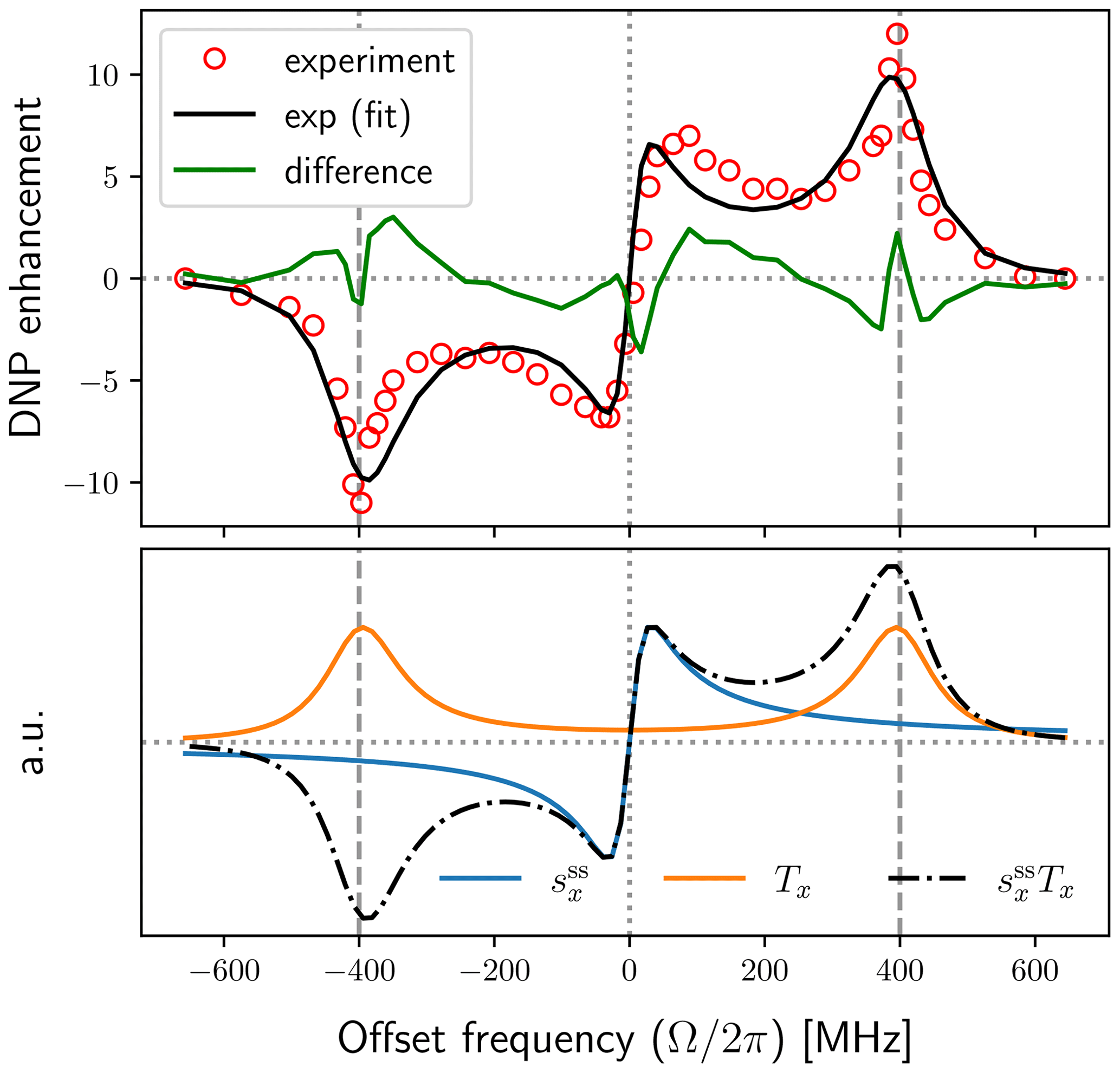
The top plot in Fig. 7 shows the experimental enhancements (red circles) together with the best fit obtained using the FFHS model with B1=6 G (solid black line). The solid green line in this plot is the difference between the experimental data and the fit. The corresponding fitting parameters are shown in the first row of Table 1. Note that the fits were performed numerically using the exact expressions of p, v±, and the DNP enhancement (Eq. 9) and were not restricted to the dependencies on the fitting parameters ri () that are indicated in Eq. (88). (For example, the general dependence of the electronic polarization factor p on T1S and T2S is not limited to the ratio .)
After the fits converged, we used the final values of the fitting parameters to calculate the dispersive component of the EPR line , and the factor Tx, such that . These are shown in the lower plot of Fig. 7, where (blue) and Tx (orange) are scaled independently along the vertical axis. Their product (dotted–dashed black line) is also scaled independently along the y axis. Since pX≈1 in our case, the product pv− is itself proportional to the solid-effect enhancement. Hence the black lines in the upper and lower plots of Fig. 7 are directly comparable. We can thus visually conclude that the unusual enhancement peaks at small offsets are a direct manifestation of the dispersive component of the power-broadened EPR line.
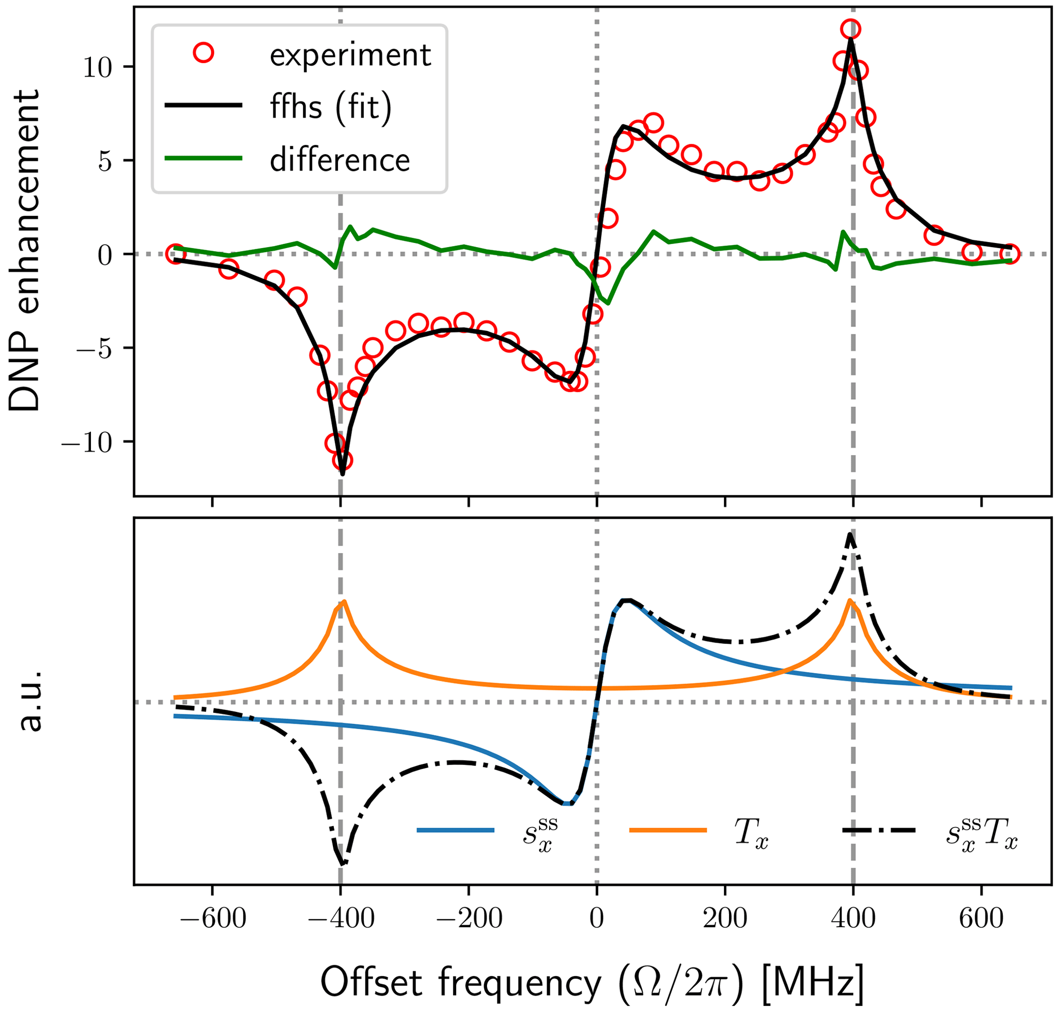
Figure 7Experimental DNP field profile at J band (red circles) and fit with the FFHS model using B1=6 G (solid black line). The central peaks in the enhancement profile follow the dispersive component of the power-broadened EPR line (solid blue line).
Table 1Fitting parameters ri () and implied timescales (T1S and τ) and contact distance (b). For different mw fields, r1 changes such that remains constant.
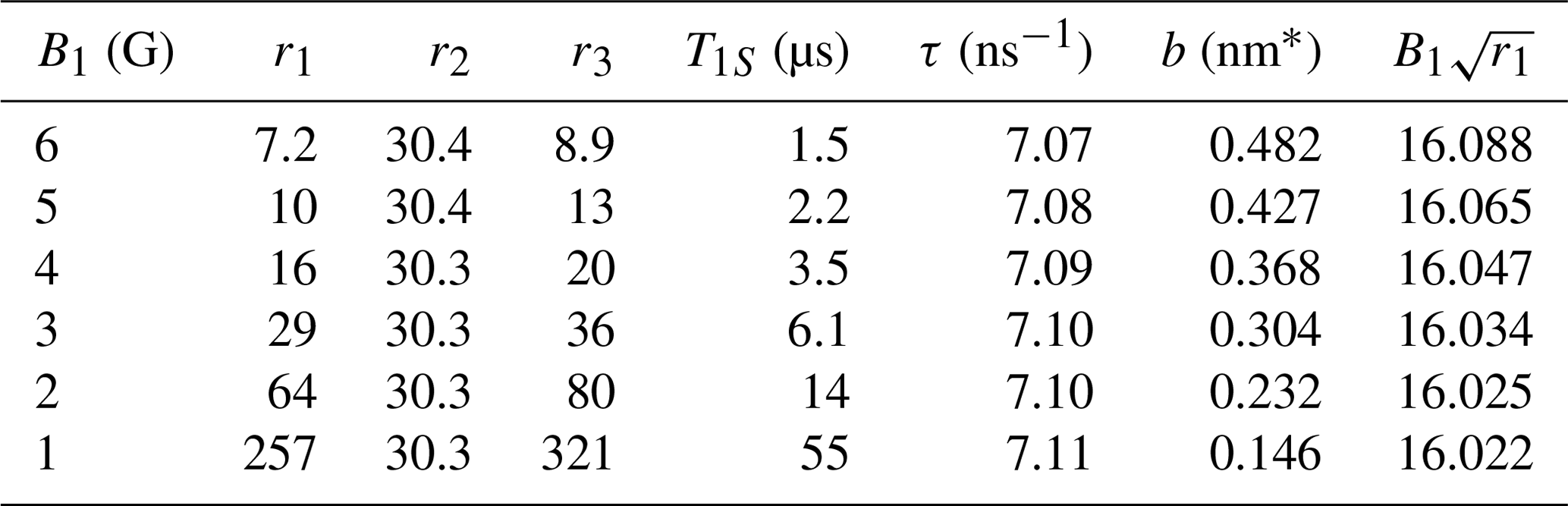
* Assuming radical concentration N=0.1 M.
Because the mw field in the experiment is not known precisely, we also attempted fits with smaller B1. The best fits were practically identical to the one shown in Fig. 7 but with different values of the fitting parameters (Table 1). (The fit for B1=2 G is shown in Fig. A1 as an example.)
From Table 1 we see that all fits resulted in the same value of the parameter r2, implying τ=7.1 ns for the motional timescale of the FFHS model. This parameter is very robust because it directly reflects the width of the experimental solid-effect lines at . Although, normally, their line width should depend on both T2S and τ, the exceptionally narrow EPR line puts us in the regime τ≪T2S where the influence of T2S is negligible. As a result, the motional broadening of the solid-effect lines in the DNP spectrum reports directly on the diffusive timescale of BDPA in the lipid environment.
The fitting parameter r1 adjusts the extrema of the dispersive EPR line (solid blue line in Fig. 7), which are at (Eq. 82). By monitoring the product of and B1 in the last column of Table 1, we see that, each time B1 is modified, the fitted r1 changes such that remains unchanged, as required by the positions of the non-canonical enhancement peaks in the experimental data. However, because r1 has to increase quadratically to compensate for the reduction of B1, the implied electronic T1 times become exceedingly long (tens of microseconds) at the smaller values of B1 (1–2 G).
When B1 is reduced, the fitting parameter r3 also increases quadratically to compensate for the dependence of the overall enhancement on . Assuming Nref=0.1 M is a good estimate of the actual concentration of BDPA in the lipid bilayer, it is possible to calculate a contact distance, b, from the fitted value of r3. The deduced contact distances are given in the second last column of Table 1. Only the values for large B1 (5–6 G) are in qualitative agreement with the molecular structure of BDPA.

Figure 8Same as Fig. 7 for the model with mono-exponential dipolar correlation function and B1=6 G (solid black line). The fit parameters r1=3.6, r2=89 and r3=7.7 correspond to T1S=0.77 µs, τ=2.4 ns and b=0.507 nm (assuming N=0.1 M).
In Fig. 8 we show a fit to the same experimental data using a mono-exponential dipolar correlation function. While the difference between the data and the fit (green line in top panel of Fig. 8) is not much worse than what we had for the FFHS model, it is apparent that the exponential model strives to find the right balance between the broadening of the solid-effect lines and the tails of these lines at the lower offsets, ultimately producing too broad solid-effect lines and too narrow non-canonical peaks. (An exponential fit with B1=4 G is shown in Fig. A2.) We thus see that the J-band DNP spectrum clearly differentiates between two alternative motional models, ruling out the less realistic one.
The most certain outcome of the fits with the FFHS model is the deduced motional timescale τ, as it comes directly from the width of the solid-effect lines (T2S is too long to contribute). The deduced value of T1S is somewhat less certain since it is accessed relative to T2S and also depends on the mw field B1. Nevertheless, with reasonable choices of T2S and B1, the fit to the non-canonical extrema in the DNP spectrum restricts T1S to a meaningful window between 1.5 and 2.5 µs (Table 1). Least certain is the estimate of the contact distance b since, in addition to B1, it requires precise knowledge of the radical concentration and the nuclear spin-lattice relaxation time. Although the latter is accessible experimentally, its value was measured at 298 K, while the DNP measurements are at 320 K.
In spite of the uncertainty in the estimated value of the distance parameter b, let us use τ and b in Eq. (67) to calculate the coefficient of relative translational diffusion. With b=0.482 nm (Table 1, first row) and τ=7.1 ns, we get . Alternatively, with b=0.427 nm (Table 1, second row) and τ=7.1 ns, we find . The first value corresponds to B1=6 G and the second to B1=5 G.
For comparison, the coefficient of lateral diffusion of phospholipids in oriented DMPC bilayers, as determined from pulsed field gradient NMR, is about at 308 K, at 323 K and at 333 K (Filippov et al., 2003, Fig. 5b, 0 mol % cholesterol). As the temperature of the DNP measurements is closer to the middle value, our two estimates of D are seen to be larger by a factor of 1.65 and 1.3, respectively.
However, the D of the FFHS model corresponds to the relative translational diffusion of the electronic and nuclear spins, i.e., , where DS and DI denote the coefficients of translational diffusion of the two spin types. Disregarding all complicating factors, one could thus take from the literature value and rationalize the values that we deduced from the width of the solid-effect DNP lines as implying either or for the diffusion coefficient of the free radical BDPA in the lipid bilayer. As the obtained numerical values are rather plausible, we conclude that the quantitative analysis of the J-band DNP spectrum leads to meaningful molecular properties. Without the theoretical framework developed in this paper, neither the molecular distance b nor the diffusion coefficient D would be accessible from a solid-effect DNP spectrum in the liquid state.
Erb, Motchane and Uebersfeld had the hunch that the dispersive component of the EPR line is reflected in the solid-effect DNP enhancement (Erb et al., 1958a). A theoretical justification of their intuition was provided in the companion paper (Sezer, 2023a). Here, the formalism was extended to the solid effect in liquids. Our theoretical predictions were compared with recent DNP measurements at high field (Kuzhelev et al., 2022). The comparison demonstrated that, under appropriate conditions, the dispersive component of the EPR line is literally visible in the field profile of the DNP enhancement. Provided that seeing is believing, we have thus closed the circle.
The DNP mechanism which became known as the solid-state effect due to Abragam (Abragam and Proctor, 1958) had been observed in liquids from the very beginning (Erb et al., 1958a, b). Nevertheless, perhaps because it yielded comparatively smaller absolute enhancements and often coexisted with the Overhauser effect (Leblond et al., 1971b), the solid effect has remained less explored in liquids compared to solids. The recent use of this DNP mechanism as a new modality for probing the molecular dynamics in ionic liquids (Neudert et al., 2017; Gizatullin et al., 2021b) and its first applications at high magnetic field (Kuzhelev et al., 2022) indicate that the potential of the solid effect in the liquid state is yet to be harvested. A theoretical understanding of the mechanism in liquids is clearly going to be helpful in these endeavors. Developing the needed theory has been the main aim of the companion and current papers.
Admittedly, a theoretical description of the solid effect in liquids was developed more than 50 years ago by Korringa and colleagues (Papon et al., 1968; Leblond et al., 1971a). In fact, their analysis was much more ambitious than ours, as it aimed to quantify the DNP spectrum during the transition from the Overhauser effect to the solid effect upon reduction of the experimental temperature (Leblond et al., 1971b). Thus, in addition to the secular terms of the dipolar interaction that we considered here and in Sezer (2023a), their Hamiltonian also contained the non-secular terms, which are important for the cross-relaxation rates of the Overhauser effect, as well as the orientation-dependent part of the electronic Zeeman interaction, which determines the electronic relaxation rates and thus the degree of saturation. Following the prescription of second-order time-dependent perturbation theory, Korringa et al. derived equations for the deviations of both the electronic and nuclear polarizations from their values at thermal equilibrium (Papon et al., 1968).
The analytical framework of Korringa and colleagues had two additional aspects. First, as is well known, the semi-classical description of spin-lattice relaxation relaxes the system to infinite temperature. The usual way of correcting for this shortcoming in magnetic resonance is to subtract the correct thermal equilibrium from the right-hand side of the dynamical equation of the density matrix (Abragam, 1961). Instead, Korringa (1964) imposed the correct temperature by writing the equation of motion of the density matrix for complex-valued time, whose imaginary part was proportional to the inverse temperature. This mathematical trick exploits the fact that a quantum-mechanical propagator with imaginary time becomes a Boltzmann factor. The analytical continuation to complex time modified the familiar Liouville–von Neumann equation of the density matrix to a form that is not common in magnetic resonance. Second, as an integral part of their formalism, Korringa et al. (1964) modeled the stochastic modulation of the spin Hamiltonian as rotational diffusion of one coordinate frame with respect to another, which led to an exponential correlation function with single decay time τ. It is not straightforward to see how their final analytical expressions should be modified if one were to use the FFHS model, for example.
In this context, it is worth mentioning that the mono-exponential model did not accurately fit the experimental data of Leblond et al. (1971b), and the authors took a Gaussian distribution for ln τ (Leblond et al., 1971a). In Fig. 8 we also observed that an exponential motional model did not fit the experimental DNP spectrum at J band (Kuzhelev et al., 2022), whereas the FFHS model with a single motional parameter did (Fig. 7). One should remember, however, that the analysis of Leblond et al. (1971b) was performed 4 years before the spectral density of the FFHS model was solved analytically (Ayant et al., 1975; Hwang and Freed, 1975).
In spite of the differences between the analytical framework of Korringa and colleagues (Papon et al., 1968; Leblond et al., 1971a) and our approach, which hamper a direct comparison of the results, we observe that the derivations in their first paper (Papon et al., 1968) assumed isotropic electronic relaxation, i.e., T1S=T2S. As we saw in Sect. 4.2, in this case the matrix 𝔅 (Eq. 13) becomes equal to 𝔅0 (Eq. 69) and the eigenvalue problem of the latter has a simple closed-form solution. All quantities of interest then become linear combinations of the reciprocals of the eigenvalues. Indeed, the final expressions of Papon et al. (1968) are linear combinations of Lorentzian spectral densities, which contain the effective frequency ωeff (Eq. 71).
The assumption of equal longitudinal and transverse electronic relaxation rates was relaxed in the second paper (Leblond et al., 1971a). Sadly, this second paper has been cited only five times, and although all of the citing papers report new experiments, they do not use the theoretical expressions of Leblond et al. (1971a) to analyze the experimental data. One can only hope that, by being less ambitious, the theory developed in the current paper fares differently.

The code used to generate the figures is at https://github.com/dzsezer/solidDNPliquids (https://doi.org/10.5281/zenodo.7990757, Sezer, 2023b).
The analyzed data are at https://github.com/dzsezer/solidDNPliquids/data (https://doi.org/10.5281/zenodo.7990757, Sezer, 2023b).
The author has declared that there are no competing interests.
Publisher’s note: Copernicus Publications remains neutral with regard to jurisdictional claims in published maps and institutional affiliations.
Andrei Kuzhelev kindly provided the analyzed experimental data in electronic form. The initial stage of the reported research was funded by grants to Thomas Prisner. Stimulating discussions with all members of the Prisner group are gratefully acknowledged.
This research has been supported by the Deutsche Forschungsgemeinschaft (grant no. 405972957).
This open-access publication was funded by the Goethe University Frankfurt.
This paper was edited by Geoffrey Bodenhausen and reviewed by Gunnar Jeschke and one anonymous referee.
Abragam, A.: The Principles of Nuclear Magnetism, Oxford University Press, New York, ISBN 978 0 19 852014 6, 1961. a, b, c
Abragam, A. and Proctor, W. G.: Une nouvelle méthode de polarisation dynamique des noyaux atomiques dans les solides, Compt. rend., 246, 2253–2256, 1958. a
Anderson, P. W.: A Mathematical Model for the Narrowing of Spectral Lines by Exchange or Motion, J. Phys. Soc. Jpn., 9, 316–339, https://doi.org/10.1143/JPSJ.9.316, 1954. a
Ayant, Y., Belorizky, E., Alizon, J., and Gallice, J.: Calcul des densit'es spectrales r'esultant d'un mouvement al'eatoire de translation en relaxation par interaction dipolaire magn'etique dans les liquides, J. Phys., 36, 991–1004, 1975. a, b, c, d, e
Delage-Laurin, L., Palani, R. S., Golota, N., Mardini, M., Ouyang, Y., Tan, K. O., Swager, T. M., and Griffin, R. G.: Overhauser Dynamic Nuclear Polarization with Selectively Deuterated BDPA Radicals, J. Am. Chem. Soc., 143, 20281–20290, https://doi.org/10.1021/jacs.1c09406, 2021. a
Denysenkov, V., Dai, D., and Prisner, T. F.: A triple resonance (e, 1H, 13C) probehead for liquid-state DNP experiments at 9.4 Tesla, J. Magn. Reson., 337, 107185, https://doi.org/10.1016/j.jmr.2022.107185, 2022. a
Eills, J., Budker, D., Cavagnero, S., Chekmenev, E. Y., Elliott, S. J., Jannin, S., Lesage, A., Matysik, J., Meersmann, T., Prisner, T., Reimer, J. A., Yang, H., and Koptyug, I. V.: Spin Hyperpolarization in Modern Magnetic Resonance, Chem. Rev., 123, 1417–1551, https://doi.org/10.1021/acs.chemrev.2c00534, 2023. a
Erb, E., Motchane, J.-L., and Uebersfeld, J.: Effet de polarisation nucléaire dans les liquides et les gaz adsorbés sur les charbons, Compt. Rend., 246, 2121–2123, 1958a. a, b
Erb, E., Motchane, J.-L., and Uebersfeld, J.: Sur une nouvelle méthode de polarisation nucléaire dans les fluides adsorbés sur les charbons, extension aux solides et en particulier aux substances organiques irradiées, Compt. Rend., 246, 3050–3052, 1958b. a
Filippov, A., Orädd, G., and Lindblom, G.: The Effect of Cholesterol on the Lateral Diffusion of Phospholipids in Oriented Bilayers, Biophys. J., 84, 3079–3086, https://doi.org/10.1016/S0006-3495(03)70033-2, 2003. a
Franck, J. M., Pavlova, A., Scott, J. A., and Han, S.: Quantitative cw Overhauser effect dynamic nuclear polarization for the analysis of local water dynamics, Prog. Nucl. Mag. Res. Sp., 74, 33–56, https://doi.org/10.1016/j.pnmrs.2013.06.001, 2013. a
Gamliel, D. and Levanon, H.: Stochastic Processes in Magnetic Resonance, World Scientific, Singapore, ISBN 978-981-283-104-0, 1995. a
Gizatullin, B., Mattea, C., and Stapf, S.: Hyperpolarization by DNP and Molecular Dynamics: Eliminating the Radical Contribution in NMR Relaxation Studies, J. Phys. Chem. B, 123, 9963–9970, https://doi.org/10.1021/acs.jpcb.9b03246, 2019. a
Gizatullin, B., Mattea, C., and Stapf, S.: Field-cycling NMR and DNP – A friendship with benefits, J. Magn. Reson., 322, 106851, https://doi.org/10.1016/j.jmr.2020.106851, 2021a. a
Gizatullin, B., Mattea, C., and Stapf, S.: Molecular Dynamics in Ionic Liquid/Radical Systems, The Journal of Physical Chemistry B, 125, 4850–4862, https://doi.org/10.1021/acs.jpcb.1c02118, 2021b. a, b, c, d
Gizatullin, B., Mattea, C., and Stapf, S.: Three mechanisms of room temperature dynamic nuclear polarization occur simultaneously in an ionic liquid, Phys. Chem. Chem. Phys., 24, 27004–27008, https://doi.org/10.1039/D2CP03437A, 2022. a, b, c
Greenwood, A. I., Tristram-Nagle, S., and Nagle, J. F.: Partial molecular volumes of lipids and cholesterol, Chem. Phys. Lipids, 143, 1–10, https://doi.org/10.1016/j.chemphyslip.2006.04.002, 2006. a
Holz, M., Heil, S. R., and Sacco, A.: Temperature-dependent self-diffusion coefficients of water and six selected molecular liquids for calibration in accurate 1H NMR PFG measurements, Phys. Chem. Chem. Phys., 2, 4740–4742, 2000. a
Hovav, Y., Feintuch, A., and Vega, S.: Theoretical aspects of dynamic nuclear polarization in the solid state – The solid effect, J. Magn. Reson., 207, 176–189, https://doi.org/10.1016/j.jmr.2010.10.016, 2010. a, b
Hwang, L.-P. and Freed, J. H.: Dynamic effects of pair correlation functions on spin relaxation by translational diffusion in liquids, J. Chem. Phys., 63, 4017–4025, 1975. a, b, c
Jakdetchai, O., Denysenkov, V., Becker-Baldus, J., Dutagaci, B., Prisner, T. F., and Glaubitz, C.: Dynamic Nuclear Polarization-Enhanced NMR on Aligned Lipid Bilayers at Ambient Temperature, J. Am. Chem. Soc., 136, 15533–15536, https://doi.org/10.1021/ja509799s, 2014. a
Korringa, J.: Dynamical Decomposition of a Large System, Phys. Rev., 133, A1228–A1229, https://doi.org/10.1103/PhysRev.133.A1228, 1964. a
Korringa, J., Motchane, J. L., Papon, P., and Yoshimori, A.: Derivation of the Modified Bloch Equations for Spin Systems, Phys. Rev., 133, A1230–A1234, https://doi.org/10.1103/PhysRev.133.A1230, 1964. a
Kubo, R.: Note on the Stochastic Theory of Resonance Absorption, J. Phys. Soc. Jpn., 9, 935–944, https://doi.org/10.1143/JPSJ.9.935, 1954. a
Kubo, R.: A stochastic theory of line shape, in: Advances in Chemical Physics, Vol. XV, edited by: Shuler, K. E., John Wiley & Sons. Inc., Chap. 6, 101–127, https://doi.org/10.1002/9780470143605.ch6, 1969. a, b, c
Kuprov, I.: Fokker-Planck formalism in magnetic resonance simulations, J. Magn. Reson., 270, 124–135, https://doi.org/10.1016/j.jmr.2016.07.005, 2016. a
Kuzhelev, A. A., Dai, D., Denysenkov, V., and Prisner, T. F.: Solid-like Dynamic Nuclear Polarization Observed in the Fluid Phase of Lipid Bilayers at 9.4 T, J. Am. Chem. Soc., 144, 1164–1168, https://doi.org/10.1021/jacs.1c12837, 2022. a, b, c, d, e, f, g, h, i, j, k, l, m, n, o, p, q
Leblond, J., Papon, P., and Korringa, J.: Stochastic Theory of Dynamic Spin Polarization in Viscous Liquids with Anisotropic Electron-Spin Relaxation, Phys. Rev. A, 4, 1539–1549, https://doi.org/10.1103/PhysRevA.4.1539, 1971a. a, b, c, d, e, f
Leblond, J., Uebersfeld, J., and Korringa, J.: Study of the Liquid-State Dynamics by Means of Magnetic Resonance and Dynamic Polarization, Phys. Rev. A, 4, 1532–1539, https://doi.org/10.1103/PhysRevA.4.1532, 1971b. a, b, c, d, e
Neudert, O., Mattea, C., and Stapf, S.: A compact X-Band resonator for DNP-enhanced Fast-Field-Cycling NMR, J. Magn. Reson., 271, 7–14, https://doi.org/10.1016/j.jmr.2016.08.002, 2016. a
Neudert, O., Mattea, C., and Stapf, S.: Molecular dynamics-based selectivity for Fast-Field-Cycling relaxometry by Overhauser and solid effect dynamic nuclear polarization, J. Magn. Reson., 276, 113–121, https://doi.org/10.1016/j.jmr.2017.01.013, 2017. a, b, c, d
Ni, Q. Z., Daviso, E., Can, T. V., Markhasin, E., Jawla, S. K., Swager, T. M., Temkin, R. J., Herzfeld, J., and Griffin, R. G.: High Frequency Dynamic Nuclear Polarization, Account. Chem. Res., 46, 1933–1941, https://doi.org/10.1021/ar300348n, 2013. a
Okuno, Y., Schwieters, C. D., Yang, Z., and Clore, G. M.: Theory and Applications of Nitroxide-based Paramagnetic Cosolutes for Probing Intermolecular and Electrostatic Interactions on Protein Surfaces, J. Am. Chem. Soc., 144, 21371–21388, https://doi.org/10.1021/jacs.2c10035, 2022. a
Papon, P., Motchane, J. L., and Korringa, J.: Unitary Theory of Dynamic Polarization of Nuclear Spins in Liquids and Solids, Phys. Rev., 175, 641–649, https://doi.org/10.1103/PhysRev.175.641, 1968. a, b, c, d, e, f
Pinon, A. C., Capozzi, A., and Ardenkjær-Larsen, J. H.: Hyperpolarization via dissolution dynamic nuclear polarization: new technological and methodological advances, Magnetic Resonance Materials in Physics, Biol. Med., 34, 5–23, https://doi.org/10.1007/s10334-020-00894-w, 2021. a
Prisner, T., Denysenkov, V., and Sezer, D.: Liquid state DNP at high magnetic fields: Instrumentation, experimental results and atomistic modelling by molecular dynamics simulations, J. Magn. Reson., 264, 68–77, https://doi.org/10.1016/j.jmr.2015.11.004, 2016. a
Sezer, D.: Non-perturbative treatment of the solid effect of dynamic nuclear polarization, Magn. Reson., 4, 129–152, https://doi.org/10.5194/mr-4-129-2023, 2023a. a, b, c, d, e, f, g, h, i, j, k, l, m, n, o
Sezer, D.: dzsezer/solidDNPliquids: v1.0 (v1.0), Zenodo [data set and code], https://doi.org/10.5281/zenodo.7990757, 2023b. a, b
Smith, A. A., Corzilius, B., Barnes, A. B., Maly, T., and Griffin, R. G.: Solid effect dynamic nuclear polarization and polarization pathways, J. Chem. Phys., 136, 015101, https://doi.org/10.1063/1.3670019, 2012. a
Tan, K. O., Mardini, M., Yang, C., Ardenkjær-Larsen, J. H., and Griffin, R. G.: Three-spin solid effect and the spin diffusion barrier in amorphous solids, Sci. Adv., 5, eaax2743, https://doi.org/10.1126/sciadv.aax2743, 2019. a
Tomlinson, D. J.: Temperature dependent self-diffusion coefficient measurements of glycerol by the pulsed N.M.R. technique, Mol. Phys., 25, 735–738, https://doi.org/10.1080/00268977300100661, 1973. a
Wenckebach, T.: Essentials of Dynamic Nuclear Polarization, Spindrift Publications, the Netherlands, ISBN 9789075541182, 2016. a, b
Wenckebach, W. T.: Electron Spin–Spin Interactions in DNP: Thermal Mixing vs. the Cross Effect, Appl. Magn. Reson., 52, 731–748, https://doi.org/10.1007/s00723-021-01335-0, 2021. a
Wiśniewski, D., Karabanov, A., Lesanovsky, I., and Köckenberger, W.: Solid effect DNP polarization dynamics in a system of many spins, J. Magn. Reson., 264, 30–38, https://doi.org/10.1016/j.jmr.2016.01.016, 2016. a