the Creative Commons Attribution 4.0 License.
the Creative Commons Attribution 4.0 License.
 | 15 Mar 2023
Multidimensional encoding of restricted and anisotropic diffusion by double rotation of the q vector
Hong Jiang
Leo Svenningsson
Daniel Topgaard
Diffusion NMR and MRI methods building on the classic pulsed gradient spin-echo sequence are sensitive to many aspects of translational motion, including time and frequency dependence (“restriction”), anisotropy, and flow, leading to ambiguities when interpreting experimental data from complex heterogeneous materials such as living biological tissues. While the oscillating gradient technique specifically targets frequency dependence and permits control of the sensitivity to flow, tensor-valued encoding enables investigations of anisotropy in orientationally disordered materials. Here, we propose a simple scheme derived from the “double-rotation” technique in solid-state NMR to generate a family of modulated gradient waveforms allowing for comprehensive exploration of the 2D frequency–anisotropy space and convenient investigation of both restricted and anisotropic diffusion with a single multidimensional acquisition protocol, thereby combining the desirable characteristics of the oscillating gradient and tensor-valued encoding techniques. The method is demonstrated by measuring multicomponent isotropic Gaussian diffusion in simple liquids, anisotropic Gaussian diffusion in a polydomain lyotropic liquid crystal, and restricted diffusion in a yeast cell sediment.
- Article
(3677 KB) - Full-text XML
-
Supplement
(294 KB) - BibTeX
- EndNote


Magnetic field gradients applied during the dephasing and rephasing periods of a spin-echo sequence (Hahn, 1950) render the NMR signal sensitive to various aspects of translational motion including bulk diffusivity (Douglass and McCall, 1958), flow (Carr and Purcell, 1954), time and frequency dependence (“restriction”) (Woessner, 1963), anisotropy (Boss and Stejskal, 1965), and exchange (Kärger, 1969). Although the conventional and ubiquitous pulsed gradient spin-echo sequence by Stejskal and Tanner (1965) may give information about all of these aspects, more elaborate gradient modulations (Tanner, 1979; Cory et al., 1990; Callaghan and Manz, 1994; Mori and van Zijl, 1995) are required to unambiguously assign a certain mechanism to the experimental observations (Topgaard, 2017; Lundell and Lasič, 2020). Diffusion MRI methods incorporating such advanced diffusion encoding schemes have recently been shown to have potential for clinical research applications (Reymbaut et al., 2020); some notable examples are oscillating gradients to estimate cell sizes (Xu et al., 2021) and tensor-valued encoding to characterize cell shapes (Daimiel Naranjo et al., 2021) in breast tumors.
The sensitivity of the MRI signal to the various types of motion can be quantified with the tensor-valued encoding spectrum b(ω) (Topgaard, 2019a; Lundell and Lasič, 2020), the trace of which equals the dephasing power spectrum (Stepišnik, 1981) – relevant for isotropic restricted diffusion – and whose integral over ω equals the conventional b matrix (Basser et al., 1994) giving information about diffusion anisotropy. While most studies focus on either the frequency-dependent (Aggarwal, 2020) or tensorial (Reymbaut, 2020) aspects of the encoding, Lundell et al. (2019) suggested joining them into a common multidimensional framework. The approach was demonstrated with gradient waveforms deriving from the magic-angle spinning (MAS) technique in solid-state NMR spectroscopy (Andrew et al., 1959; Eriksson et al., 2013; Topgaard, 2013); however, these methods offer only limited access to the frequency and anisotropy dimensions.
Expanding on the results of Lundell et al. (2019), we take inspiration from the “double-rotation” (DOR) technique in solid-state NMR (Samoson et al., 1998) and derive a family of gradient waveforms for comprehensive exploration of, in particular, the frequency–anisotropy dimensions of b(ω), as quantified by the centroid frequency ωcent (Arbabi et al., 2020) and encoding anisotropy bΔ (Eriksson et al., 2015), in addition to the b value and b vector (Θ, Φ) of conventional diffusion tensor imaging (Kingsley, 2006). While ωcent is key for characterizing restricted diffusion (Stepišnik and Callaghan, 2000), the variable bΔ enables quantification of anisotropy in orientationally disordered materials (Eriksson et al., 2015) and estimation of nonparametric diffusion tensor distributions (de Almeida Martins and Topgaard, 2016; Topgaard, 2019b). The ability of the new gradient waveforms to give access to the complete 2D ωcent–bΔ plane is demonstrated by microimaging measurements on previously studied phantoms with well-defined restriction and anisotropy properties, namely water (Mills, 1973) and concentrated salt solution (Wadsö et al., 2009) with isotropic Gaussian diffusion, a lamellar liquid crystal giving anisotropic Gaussian diffusion (Topgaard, 2016), and a yeast cell sediment exhibiting isotropic restricted diffusion (Malmborg et al., 2006).
To set the stage for later sections dealing with the proposed gradient waveforms to investigate both frequency-dependent and tensorial aspects of translational motion, we include a brief summary of the relevant theory here; greater detail can be found in the textbooks by Price (2009) and Callaghan (2011) as well as in the comprehensive review by Lundell and Lasič (2020). Readers already familiar with the background material may proceed directly to the design of gradient waveforms in Sect. 3 after noting Eqs. (32) and (34) with the definitions of the main variables ωcent and bΔ reporting on the sensitivity to restriction and anisotropy.
2.1 Encoding of translational motion by magnetic field gradients
Figure 1 illustrates the effects of a general gradient waveform g(t) on the NMR signal from an ensemble of spins undergoing restricted diffusion and flow within an infinite cylinder. As shown using the 2D and 3D plots of g(t) in Fig. 1a, both the magnitude and direction of the gradient vector are changing smoothly with time. Simultaneously, the spins spread out and gradually drift from their initial positions (Fig. 1b). The time-dependent normalized signal E(t) is given by
where 〈…〉 denotes an ensemble mean and the time-dependent phase ϕ(t) of a single spin with gyromagnetic ratio γ is determined by the time integral of the scalar product between g(t) the time-dependent position r(t) according to
The interplay between g(t) and r(t) results in ϕ(t) evolving from zero for all spins at t=0 to periodic patterns with varying directions and spatial wavelengths at intermediate times and, finally, an overall phase shift superposed on partially randomized values. From Eq. (1), it follows that the latter phase dispersion leads to a decrease in the magnitude of the signal.
The evolution of ϕ(t) may be rationalized by partial integration of Eq. (2) into
where q(t) is the dephasing vector, defined as
and v(t) = dr(t) dt is the time-dependent velocity. The spatial periodicity in ϕ(t) at intermediate times is, according to the first term in Eq. (3), given by the scalar product between q(t) and r(t), which is utilized to obtain the spatial resolution in MRI where the dephasing vector is usually denoted k(t). The plots of q(t) in Fig. 1a show smooth changes in both the magnitude and direction of the vector with time.
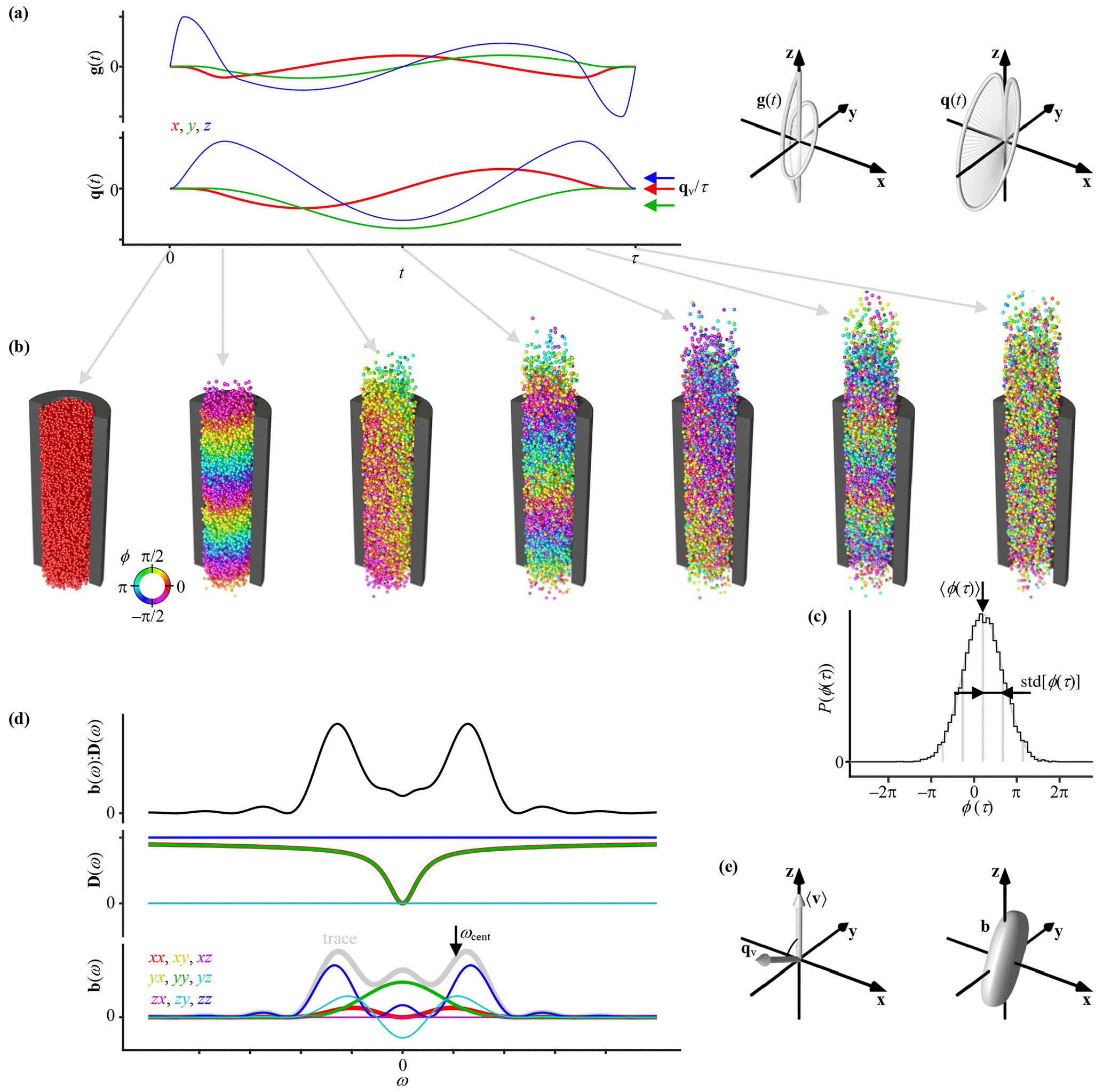
Figure 1Principles of motion encoding by general gradient waveforms. (a) Time-dependent gradient g(t) and dephasing vector q(t) illustrated as 2D graphs of Cartesian components vs. t (left) and 3D plots of trajectories through space (right). The average values of the q(t) components within the time interval from t=0 to τ are indicated with arrows labeled , where the velocity-encoding vector qv is defined in Eq. (15). (b) Sequence of snapshots from a random walk simulation of an ensemble of spins (spheres) undergoing restricted diffusion and flow within an infinite cylinder (black section) during application of the waveforms in panel (a). Each spin is color-coded by its time-dependent phase ϕ(t) given by the interplay between g(t) and the spin positions r(t) according to Eq. (2). (c) Phase distribution P(ϕ(τ)) for the ensemble of spins at t=τ (black histogram) and a Gaussian (smooth gray line) with mean 〈ϕ(τ)〉 and standard deviation std[ϕ(τ)] (spacing between vertical gray lines) which give the phase shift α and attenuation factor β of the signal E(τ) via Eqs. (8), (9), and (11). (d) Frequency-dependent elements (color-coded) of the tensor-valued encoding spectrum b(ω) and diffusion spectrum D(ω) as well as their tensor dot product b(ω) : D(ω) which gives β via Eq. (21). The centroid frequency ωcent (arrow) is obtained from the trace of b(ω) (gray line) via Eq. (32). (e) The 3D plots of the ensemble mean velocity 〈v〉, velocity-encoding vector qv, and encoding tensor b, with the latter being defined in Eq. (33). The scalar product of 〈v〉 and qv gives α via Eq. (14).
Focusing on translational displacements rather than absolute positions, we select a time τ where
and the first term in Eq. (3) vanishes while the second one remains:
The value of ϕ(τ) in Eq. (6) is insensitive to r(τ) but depends on the history of q(t) and v(t) in the interval from t=0 to τ.
2.2 Gaussian phase distribution approximation
As shown in Fig. 1c, the selected gradient waveform and random walk simulation parameters yield a phase distribution P(ϕ(t)) that is well approximated at t=τ as a Gaussian function with mean 〈ϕ(τ)〉 and standard deviation std[ϕ(τ)] = (〈ϕ(τ)2〉 – 〈ϕ(τ)〉2). The Gaussian function can be expressed as
where
and
After rewriting Eq. (1) as an integral,
the insertion of Eq. (7) into Eq. (10) may be evaluated to
where α and β can be identified as quantitative measures of the overall phase shift and attenuation of the signal, respectively, as previously deduced from visual inspection of the phases of the spin ensemble in Fig. 1b. The Gaussian phase distribution approximation has been applied for the cases of free (Carr and Purcell, 1954; Douglass and McCall, 1958) and restricted (Neuman, 1974) diffusion, and investigations of its ranges of validity can be found in the literature (Balinov et al., 1993; Stepišnik, 1999).
2.3 Mean velocity and velocity correlation function
Insertion of Eq. (6) into Eq. (8) yields
which by separating v(t) into the ensemble mean 〈v(t)〉 = 〈v〉 and fluctuating part u(t), defined by
can be evaluated to
where the flow encoding vector qv is defined as
Correspondingly, the insertion of Eq. (6) into Eq. (9) gives
which by reordering the time integrals and ensemble means as well as noting that 〈u(t) ⋅ 〈v〉〉=0, can be expressed as
where 〈u(t)u(t′)T〉 is the tensor-valued velocity correlation function.
2.4 Transformation to the frequency domain
After introducing the dephasing spectrum q(ω) and diffusion spectrum D(ω) by Fourier transformations to the frequency (ω) domain according to
and
Eq. (17) can be recast into
which can be expressed more compactly as
where b(ω) is the tensor-valued encoding spectrum defined as (Topgaard, 2019a; Lundell and Lasič, 2020)
and “:” denotes a tensor dot product (Basser et al., 1994):
Combining Eqs. (11), (14), and (21) yields
where the motion-encoding properties of g(t) are summarized in qv and b(ω), as illustrated in Fig. 1d and e. While qv and 〈v〉 are (ω-independent) vectors, both b(ω) and D(ω) are symmetric second-order tensors at each value of ω.
2.5 Diffusion spectra for some simple cases
For a liquid with bulk diffusivity D0 confined in d dimensions in planar (d=1), cylindrical (d=2), or spherical (d=3) compartments with radius r, the diffusion spectrum Drest(ω) in the restricted dimensions can be expressed as follows (Stepišnik, 1993):
where
and
Equation (25) includes the long-range diffusivity D∞, allowing for finite permeability of the compartment walls (Lasič et al., 2009), and can be recognized as a sum of Lorentzians with widths Γk and weights wk. In Eqs. (26) and (27), ξk is the kth solution of
where Jν is the νth-order Bessel function of the first kind. Using the cylindrical case in Fig. 1b as an example, the tensor-valued diffusion spectrum D(ω) is given by
where θ and ϕ are polar and azimuthal angles, giving the orientation of the cylinder in the lab frame, and R(θ, ϕ) is a rotation matrix. Figure 1d includes a plot of D(ω) for the case θ=0 and ϕ=0 where all off-diagonal elements are zero. At high values of ω, the diagonal elements converge towards D0, corresponding to isotropic diffusion. Conversely, the effects of anisotropy reach a maximum in the low-ω limit where Drest(ω) approaches D∞, which equals zero in the example in Fig. 1d. The planar version of Eq. (29) is obtained by exchanging Drest(ω) and D0. In the low-ω limit, the planar and cylindrical cases are often combined into a single expression:
where D∥ and D⊥ are the eigenvalues parallel and perpendicular to the main symmetry axis of the compartment, respectively. For completeness, we note that Drest(ω) and D in Eqs. (25) and (30), respectively, reduce to an ω-independent scalar diffusion coefficient D for the special case of isotropic Gaussian diffusion where .
2.6 Key properties of the tensor-valued diffusion encoding spectrum
While the signal expression in Eq. (24) takes the ω dependence and tensorial properties of both b(ω) and D(ω) into account and may be numerically evaluated as a single matrix multiplication after discretization in the ω dimension and appropriate reordering of the tensor elements, the common occurrence of systems exhibiting approximately Gaussian (ω-independent) and/or isotropic diffusion has led to the introduction of simplified descriptions focusing on some specific aspects. In the absence of diffusion anisotropy – which is obviously not the case for the example in Fig. 1 – it is sufficient to use the dephasing power spectrum b(ω) (Stepišnik, 1981) obtained from b(ω) by
The sensitivity to restriction can be summarized by the centroid frequency ωcent (Arbabi et al., 2020), defined as
In addition to all the tensor elements of b(ω), Fig. 1d includes a plot of b(ω) with an arrow indicating ωcent. The example of b(ω) covers both low- and high-ω features of D(ω) and is, thus, less well suited for exploring ω-dependent diffusion processes than gradient modulation schemes comprising trains of rectangular pulses (Callaghan and Stepišnik, 1995), multiple smooth oscillations (Parsons et al., 2003), or a Carr–Purcell–Meiboom–Gill sequence in the presence of a constant gradient (Lasič et al., 2006), where the encoding power is concentrated in a narrow frequency range and the single value ωcent captures most of the relevant information about the spectral content. Even when the peaks in b(ω) are broader than the features in D(ω), the ωcent metric has some value as a bookkeeping tool but is less suitable for quantitative analysis.
For anisotropic systems with Gaussian diffusion, it is useful to introduce the b-matrix b (Basser et al., 1994) by
The sensitivity to anisotropy is given by the “shape” of the tensor which can be quantified with the encoding anisotropy bΔ and asymmetry bη (Eriksson et al., 2015), defined as
and
respectively. Here, bXX, bYY, and bZZ are the eigenvalues of b ordered according to the Haeberlen convention (Haeberlen, 1976) and
is the conventional b value (Le Bihan et al., 1986) that gives the overall magnitude of the diffusion encoding. Figure 1e shows a superquadric tensor glyph (Kindlmann, 2004) representation of b where all eigenvalues and both shape parameters bΔ and bη are nonzero.
From the definitions of qv, q(ω), and b(ω) in Eqs. (15), (18), and (22), it follows that the ω=0 values of b(ω) are proportional to and, thus, report on the sensitivity to flow, albeit with some ambiguity with respect to the directionality: the vectors qv and −qv give the same b(ω=0). It should be noted that qv is not necessarily colinear with any of the eigenvectors of b.
2.7 Special cases for data analysis
For data-fitting purposes, it is convenient to write the normalized signal E as the ratio
where S is detected signal and S0 is the signal obtained in a reference measurement with the amplitudes of the motion-encoding gradients set to zero. Equation (24) can then be expressed as
For the special cases of (i) isotropic restricted, (ii) anisotropic Gaussian, and (iii) isotropic Gaussian diffusion in the absence of net flow (〈v〉=0), Eq. (38) is simplified to
and
respectively, where D(ω) is the (isotropic) diffusion spectrum, D is the (ω-independent) diffusion tensor, and D is the (isotropic and ω-independent) diffusion coefficient introduced in Sect. 2.5 above.
For a heterogeneous system including multiple sub-ensembles i with individual signals Si, each of which is given by one of the equations (Eqs. 38–41) above, the total signal S is obtained by the sum
An important type of heterogeneity refers to the orientations of anisotropic objects with the extreme case of completely random orientations as in a “powder”. In the special case of axial symmetry of both b and D, powder averaging of Eq. (40) yields (Eriksson et al., 2015)
where
In Eq. (44), Diso is the isotropic diffusivity and DΔ is the normalized diffusion anisotropy; these terms are defined as
and
respectively. Here, D∥ and D⊥ were introduced in Eq. (30). The definitions of bΔ and b can be found in Eqs. (34) and (36), respectively.
Expanding on previous magic-angle spinning (Andrew et al., 1959; Eriksson et al., 2013; Topgaard, 2013) and variable-angle spinning (Frydman et al., 1992; Topgaard, 2016, 2017) approaches for generating motion-encoding gradient waveforms, we apply the double-rotation (DOR) technique (Samoson et al., 1998; Topgaard, 2019a) to probe the 2D acquisition space spanned by the variables ωcent and bΔ defined in Eqs. (32) and (34), respectively. The q-vector trajectory q(t) is expressed in terms of its time-dependent magnitude q(t) and unit vector u(t) as
For the special case of DOR, the unit vector is written as
where Rz and Ry are Euler rotation matrices, ζ1 and ζ2 are the inclinations of the two rotation axes, and ψ1(t) and ψ2(t) are the time-dependent angles of rotation. The rotations in Eq. (48) are applied from right to left and follow a Z–Y active rotation matrix convention.
Starting from a conventional 1D gradient waveform g1D(t) – for instance, a pair of rectangular or sine-bell pulses of opposite polarity – the time-dependent functions q(t) and ψ2(t) are given by Topgaard (2016):
and
where Δψ2 is the total angle of rotation during the encoding interval from time t=0 to τ and
is the conventional b value. After some exercises in trigonometry, combination of Eqs. (47)–(51) and the relation between g(t) and q(t) in Eq. (4) yields
where
is the time-dependent magnitude of the rotating gradient vector;
are time-dependent rotation angles; and
are amplitudes of the oscillating terms.
In the solid-state NMR field, DOR is applied with the inclinations and , corresponding to zeros of the second and fourth Legendre polynomial, to eliminate both first- and second-order quadrupolar broadening of the NMR spectra of nuclei such as 23Na (Samoson et al., 1998). While the encoding anisotropy bΔ in Eq. (34) is closely related to the second Legendre polynomial (Eriksson et al., 2015), we are not yet aware of any diffusion analog of the quadrupolar interactions involving the fourth Legendre polynomial. Instead, we found that DOR with the inclinations and yields desirable properties for diffusion encoding, namely spectral content concentrated to a narrow frequency window for all of the elements of b(ω). For n>1 and the special case of g1D(t) ∝ [δ(t) − δ(t − τ)], where δ(x) is the Dirac delta function, these angles yield an isotropic b tensor, corresponding to bΔ=0. Waveforms for any values of bΔ and bη are then conveniently obtained by scaling the components of gDOR(t) according to
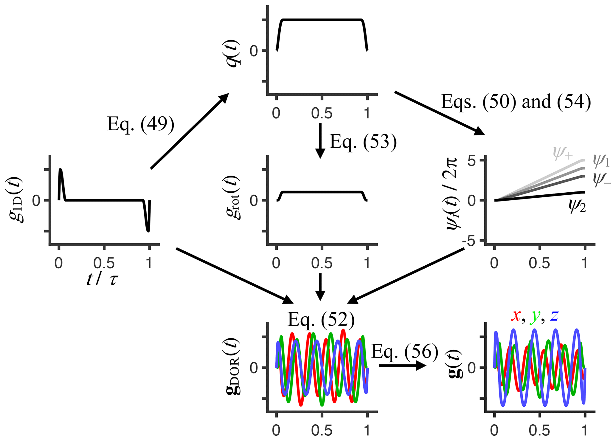
Figure 2Flowchart for calculating a double-rotation gradient waveform gDOR(t) given a 1D dephasing/rephasing waveform g1D(t), rotation axis inclinations ζ1 and ζ2, double-rotation ratio n, and total angle of rotation Δψ2 during the waveform duration τ. The waveform g1D(t), containing dephasing and rephasing pulses with sinusoidal ramps of durations εup and εdown, gives the time-dependent magnitude of the dephasing vector q(t) via Eq. (49), which yields the time-dependent rotation angles ψi(t) via Eqs. (50) and (54) as well as the time-dependent magnitude of the rotating and oscillating gradient grot(t) via Eq. (53). Combining g1D(t), grot(t), and ψi(t) via Eq. (52) gives gDOR(t), which, if and , n is an integer above 1, and Δψ2 is a multiple of 360∘, achieves isotropic encoding tensors b where the anisotropy bΔ and asymmetry bη are both equal to zero. Finally, waveforms g(t) for any values of bΔ and bη are obtained by scaling of the Cartesian components of gDOR(t) according to Eq. (56). The shown example was generated with the MATLAB code provided in the Supplement using εup=0.015τ, εdown=0.06τ, , n=4, bΔ=0.5, and bη=0.25.
At the selected inclinations, the a0 and a2 terms in Eq. (52) equal zero, while the remaining amplitudes evaluate to , , and . For the special case g1D(t) ∝ [δ(t) − δ(t − τ)], the main frequency components of b(ω) are thus given by
where, according to Eq. (52), ω± and ω1 are cleanly separated into the respective transverse (X, Y) and longitudinal (Z) directions. The mean frequency content, as quantified by the centroid frequency ωcent defined in Eq. (32), can be estimated by weighting the contributions from the main frequency components by the corresponding amplitudes in Eq. (52) but is more accurately calculated by the numerical evaluation of Eq. (32), which also takes the finite durations of the sinusoidal oscillations into account. For rough prediction of ωcent, it is useful to note that , implying that the ω+ component will dominate the spectra in the X and Y directions. The scaling of the waveforms according to Eq. (56) preserves the frequency content in each of the eigendirections of the b tensor but shifts the value of ωcent between the approximate extremes ω+ and ω1 for and 1, respectively. The differences in ω± and ω1 may give rise to a directional dependence of the sensitivity to restriction as investigated for the bΔ=0 case by de Swiet and Mitra (1996).
Figure 2 illustrates the series of calculations required to convert a conventional 1D waveform g1D(t) and given values of ζ1, ζ2, Δψ2, n, bΔ, and bη to a 3D waveform g(t) by numerical evaluation of Eqs. (49)–(56). Following previous works to generate families of smooth gradient waveforms to explore the bΔ and bη dimensions of diffusion encoding (Topgaard, 2016, 2017), we construct g1D(t) from a dephasing lobe with quarter-sine ramp-up of duration εup and half-cosine ramp-down of duration εdown as well as a rephasing lobe obtained by inversion and time-reversal of the dephasing one. The corresponding MATLAB code is provided in the Supplement.
Figure 3 compiles waveforms and encoding spectra for an array of n and bΔ at constant g1D(t), τ, and Δψ2, yielding constant b. Increasing n leads to larger rotation angles ψ1(t) and ψ±(t) and frequencies ω1 and ω± according to Eqs. (54) and (57), respectively, at the expense of overall higher gradient amplitudes on account of the terms including n in Eq. (52). For most waveforms, vanishing values of b(ω) at ω=0 correspond to qv=0 and insensitivity to flow. Many of the examples in Fig. 3 are familiar from the literature, such as conventional Stejskal–Tanner encoding at (n=0, bΔ=1), basic flow-compensated encoding (Caprihan and Fukushima, 1990) at (n=1, bΔ=1), and magic-angle spinning of the q vector (Eriksson et al., 2013) at (n=0, bΔ=0). The series of bΔ=1 and waveforms with varying n resemble the cosine-modulated oscillating gradients of Parsons et al. (2003) and the circularly polarized version introduced by Lundell et al. (2015), respectively. Correspondingly, the series of waveforms with n=0 and varying bΔ has previously been introduced as a diffusion version of the variable-angle spinning technique to correlate isotropic and anisotropic chemical shifts in solid-state NMR (Topgaard, 2016, 2017). The approach for joint investigation of restricted and anisotropic diffusion proposed by Lundell et al. (2019), combining isotropic encoding with “tuned” and “detuned” directional encodings, can be recognized as measurements at the three discrete points (n=0, bΔ=0), (n=0, bΔ=1), and (n=1, bΔ=1) of the 2D plane in Fig. 3. For completeness, we note that the elliptically polarized oscillating gradients by Nielsen et al. (2018) can be reproduced with and bη in the range from 0 to 3 (not included in Fig. 3).
Magnesium nitrate hexahydrate, cobalt nitrate hexahydrate, and 1-decanol were purchased from Sigma-Aldrich Sweden AB and sodium octanoate was obtained from J&K Scientific via Th. Geyer in Sweden. Water was purified with a Milli-Q system. A sample with two-component isotropic diffusion was prepared by inserting a 4 mm NMR tube containing an aqueous solution saturated with magnesium nitrate (Wadsö et al., 2009) into a 10 mm NMR tube with water (Mills, 1973). The magnesium nitrate solution was spiked with a small amount of cobalt nitrate (0.27 wt % saturated solution) to reduce T1 and T2 to approx. 500 and 50 ms, respectively. An anisotropic sample was prepared by mixing 85.79 wt % Milli-Q, 9.17 wt % 1-decanol, and 5.04 wt% sodium octanoate giving a lamellar liquid crystal (Persson et al., 1975). Investigation of isotropic restricted diffusion was performed with a sediment of fresh baker's yeast (trade name: Kronjäst; obtained from a local supermarket) prepared by dispersing yeast in tap water (1:1 volume ratio) in a glass vial, transferring it with a syringe to a 10 mm NMR tube to a sample height of 40 mm, and keeping the tube in an upright position overnight at 4 ∘C to allow the cells to settle under the force of gravity into a 20 mm high pellet (Malmborg et al., 2006).
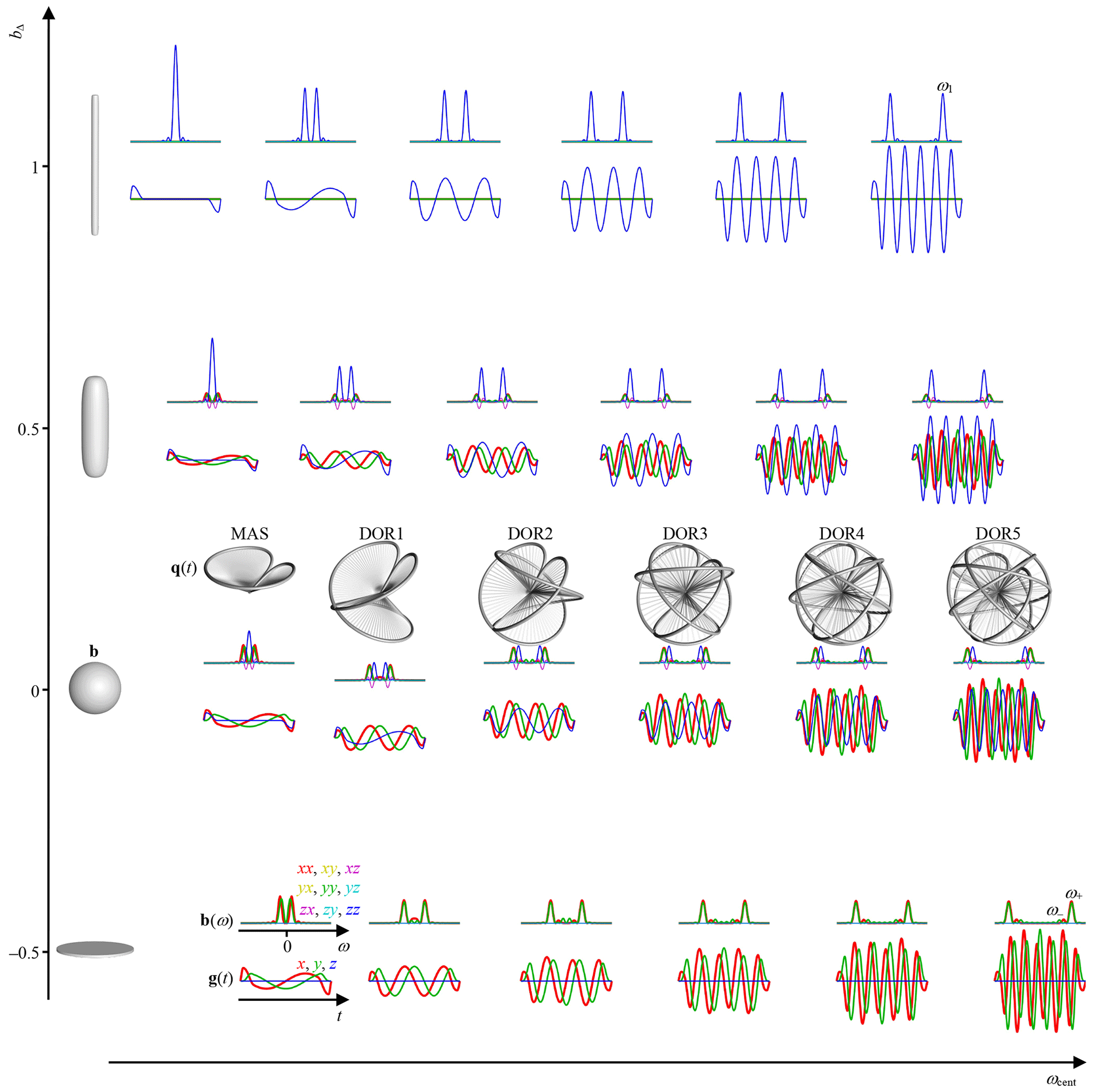
Figure 3Gradient waveforms g(t) for comprehensive exploration of the 2D space of centroid frequency ωcent and anisotropy bΔ of the tensor-valued encoding spectrum b(ω). Magic-angle spinning (MAS) and double rotation (DORn) with variable frequency ratio n give q-vector trajectories q(t) shown as 3D plots for the bΔ=0 cases. The waveforms are generated according to the scheme in Fig. 2 using εup=0.03τ, εdown=0.12τ, , bη=0, and identical b values for a 2D array of n=0, 1, …, 5 and , 0, 0.5, and 1 with the angles and for n=0 and and for n>0. Superquadric tensor glyphs (Kindlmann, 2004) along the vertical axis illustrate b for the chosen values of bΔ. The main maxima in b(ω) are located at the frequencies ω1 and ω+ given in Eq. (57). Values of ωcent and bΔ, including non-idealities originating from the finite durations of the dephasing and rephasing lobes of g1D(t), are obtained via Eqs. (32) and (34), respectively, using numerically evaluated b(ω) according to Eqs. (4), (18), and (22).
MRI was performed on a Bruker AVANCE NEO 500 MHz spectrometer equipped with an 11.7 T vertical bore magnet and a MIC-5 microimaging probe fitted with a 10 mm radiofrequency insert for observation of 1H. Images were acquired with a TopSpin 4.0 implementation of a spin-echo prepared single-shot RARE (Rapid Imaging with Refocused Echoes) sequence (available at https://github.com/daniel-topgaard/md-dmri, last access: 1 October 2022) using a 0.6 × 0.6 mm2 resolution in a plane perpendicular to the tube axis, a 1 mm slice thickness, and a 16 × 16 × 1 matrix size. Diffusion encoding employed pairs of identical gradient waveforms bracketing the 180∘ pulse in the preparation block (Lasič et al., 2014). Data were acquired for 8 b values up to 6.44⋅109 s m−2 and 15 orientations (Θ, Φ) for each of the 24 waveforms spanning the 2D ωcent–bΔ plane in Fig. 3 using a maximum gradient amplitude of 3 T m−1 and a waveform duration of τ=25 ms, giving values of ωcent in the range of 20–260 Hz. With a 5 s recycle delay, the total measurement time was approximately 4 h for each sample. The sample temperature was controlled with a Bruker VT unit: 278 K for the yeast and 291 K for the isotropic solutions and liquid crystal. For the yeast, the image slice was placed in the middle of the pellet and 10 mm below the bottom of the supernatant. Image reconstruction, definition of regions of interest, and curve fitting were performed in MATLAB using in-house code available at https://github.com/daniel-topgaard/md-dmri, last access: 1 October 2022 (Nilsson et al., 2018).
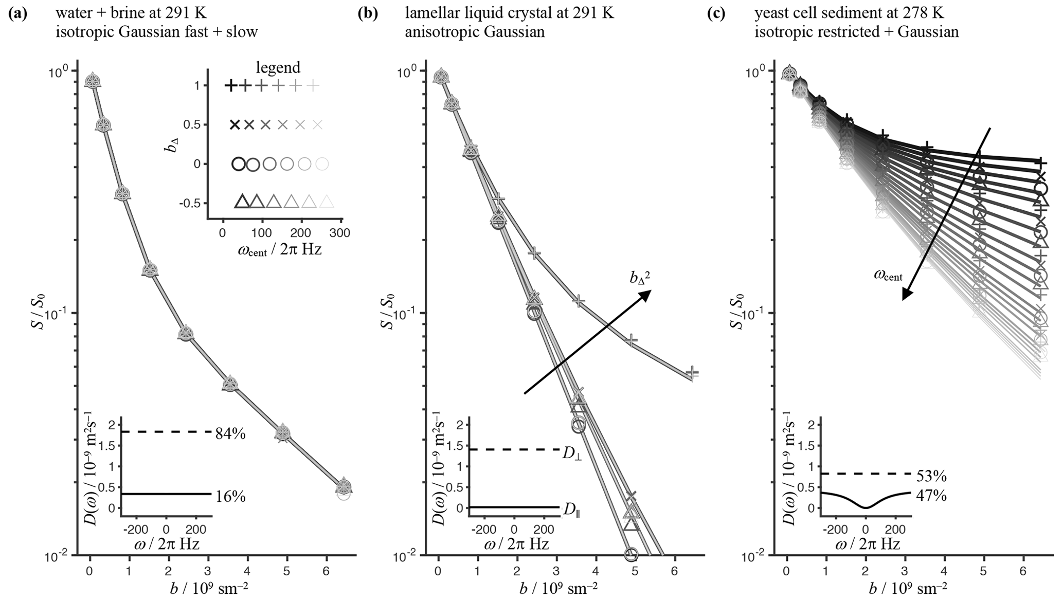
Figure 4Experimental (markers) and fitted (lines) normalized powder-averaged signal vs. b value for phantoms with well-defined diffusion properties. (a) Tube-in-tube assembly of pure water and a concentrated solution of magnesium nitrate in water (“brine”) giving rise to two isotropic Gaussian (ω-independent) components. A two-component fit based on Eq. (41) gives diffusion spectra D(ω), as shown in the inset, with percentages indicating the relative contributions. The legend shows the 24 investigated values in the 2D ωcent (the gray scale) and bΔ (marker style) space corresponding to the gradient waveforms in Fig. 3 with a duration of τ=25 ms, a maximum gradient strength of 3 Tm−1, and pairs of waveforms bracketing the 180∘ pulse in the spin-echo preparation. (b) Polydomain lamellar liquid crystal giving Gaussian parallel and perpendicular diffusivities, D∥ and D⊥, as estimated by a fit of Eq. (43). (c) Sediment of yeast cells with intra- and extracellular compartments, with the former exhibiting restricted (ω-dependent) diffusion. The inset shows D(ω) resulting from a two-component fit with one spherically restricted (solid) and one Gaussian (dashed) component. For the former component, the signal was obtained by numerical integration of Eq. (39) with D(ω) given by Eq. (25) with d=3 and D∞ constrained to zero.
Figure 4 compiles experimental data and fits for all investigated samples. To facilitate visual inspection of the highly multidimensional data acquired as a function of (b, ωcent, bΔ, Θ, Φ), the signal data were averaged over b-tensor orientations (Θ, Φ) and are displayed as conventional Stejskal–Tanner plots of log10(S) vs. b with the ωcent and bΔ dimensions coded using different marker styles and a gray scale. For the isotropic Gaussian sample in Fig. 4a, all data points collapse onto a single master curve, thereby verifying that all 24 waveforms spanning the 2D ωcent–bΔ plane in Fig. 3 indeed give the same b value. The pronounced nonlinearity of the log10(S) vs. b plot indicates the presence of multiple species with different diffusivities, and the bi-exponential fit yields diffusivities consistent with pure water (fast) and water in the saturated magnesium nitrate solution (slow). The anisotropic Gaussian phantom Fig. 4b yields data points stratified into one master curve for each of the four values of bΔ, verifying independence of ωcent. The data are well fitted by the expression for randomly oriented axisymmetric diffusion tensors in Eq. (43), giving estimates of the diffusivities D∥ and D⊥ parallel and perpendicular to the cylindrical symmetry axis of the crystallites. The observations and are consistent with diffusion in a lamellar liquid crystal with planar surfactant bilayers being nearly impermeable to water (Callaghan and Söderman, 1983). For the isotropic restriction phantom in Fig. 4c, the signal depends strongly on ωcent. In this case, there is no clear stratification of data points into separate master curves on account of the interplay between bΔ and ωcent, as reported in the legend in Fig. 4a and explained in detail below Eq. (57). The minor dependence of ωcent on bΔ is admittedly a drawback of our current approach for generating waveforms; however, we believe our approach is justified by the simplicity and transparency of the mathematical expressions in Eqs. (49)–(57). The sum of isotropic restricted and Gaussian components, given by Eqs. (41) and (39), yields an excellent fit to the acquired data, showing that the data feature no dependence on the value of bΔ. To account for the fact that b(ω) for (in particular) the bΔ=0 waveforms cannot be well approximated with a delta function at a single value of ω, the signal for the restricted component was obtained by numerical evaluation of the integral in Eq. (39) using the diffusion spectrum D(ω) for spherical compartments in Eq. (25). The obtained diffusivities are consistent with previous results for intra- and extracellular water in yeast cell sediments (Åslund and Topgaard, 2009). Taken together, the data in Fig. 4 verify that the set of waveforms allows detailed exploration of the 2D ωcent–bΔ plane of multidimensional diffusion encoding.
The proposed family of double-rotation gradient waveforms enables comprehensive sampling of both the frequency and “shape” dimensions of diffusion encoding, as required for detailed characterization of restriction and anisotropy in heterogeneous materials such as brain tissues. The present waveforms, deriving from simple geometrical considerations and generated by compact mathematical expressions, are suitable for preclinical investigations of tissue samples or small animals on high-gradient systems. By numerical optimizations to maximize the b value for given gradient strength (Topgaard, 2013; Sjölund et al., 2015), mitigating image artifacts from eddy currents (Yang and McNab, 2019) and concomitant gradients (Szczepankiewicz et al., 2019), and further minimizing side lobes in the encoding spectra (Hennel et al., 2020), we anticipate that the waveforms may be adapted for human in vivo studies. The merging of oscillating gradients (Aggarwal, 2020) and tensor-valued encoding (Reymbaut, 2020) into a common acquisition protocol encourages further development of a joint analysis framework, for instance, by augmenting current nonparametric diffusion tensor distributions (Topgaard, 2019b) with a Lorentzian frequency dimension (Narvaez et al., 2021, 2022) or building on the concept of confinement tensors (Yolcu et al., 2016; Boito et al., 2022).
MATLAB code for image reconstruction, the definition of regions of interest, and curve fitting is available from https://github.com/daniel-topgaard/md-dmri (Topgaard, 2021; Nilsson et al., 2018).
Experimental data are available from https://github.com/daniel-topgaard/md-dmri-data (Topgaard, 2021).
The supplement related to this article is available online at: https://doi.org/10.5194/mr-4-73-2023-supplement.
DT conceived the project. HJ, LS, and DT developed theory and software. HJ acquired data. HJ and DT processed and analyzed data. HJ, LS, and DT wrote the manuscript.
The contact author has declared that none of the authors has any competing interests.
Publisher’s note: Copernicus Publications remains neutral with regard to jurisdictional claims in published maps and institutional affiliations.
This research has been supported by the Swedish Foundation for Strategic Research (Stiftelsen för Strategisk Forskning; grant no. ITM17-0267), the Swedish Research Council (Vetenskapsrådet; grant nos. 2018-03697 and 2022-04422_VR), and the China Scholarship Council.
This paper was edited by Kong Ooi Tan and reviewed by Tom Barbara and one anonymous referee.
Aggarwal, M.: Restricted diffusion and spectral content of the gradient waveforms, in: Advanced Diffusion Encoding Methods in MRI, edited by: Topgaard, D., Royal Society of Chemistry, Cambridge, UK, 103–122, https://doi.org/10.1039/9781788019910-00103, 2020.
Andrew, E. R., Bradbury, A., and Eades, R. G.: Removal of dipolar broadening of nuclear magnetic resonance spectra of solids by specimen rotation, Nature, 183, 1802–1803, https://doi.org/10.1038/1831802a0, 1959.
Arbabi, A., Kai, J., Khan, A. R., and Baron, C. A.: Diffusion dispersion imaging: Mapping oscillating gradient spin-echo frequency dependence in the human brain, Magn. Reson. Med., 83, 2197–2208, https://doi.org/10.1002/mrm.28083, 2020.
Åslund, I. and Topgaard, D.: Determination of the self-diffusion coefficient of intracellular water using PGSE NMR with variable gradient pulse length, J. Magn. Reson., 201, 250–254, https://doi.org/10.1016/j.jmr.2009.09.006, 2009.
Balinov, B., Jönsson, B., Linse, P., and Söderman, O.: The NMR self-diffusion method applied to restricted diffusion. Simulation of echo attenuation from molecules in spheres and between planes, J. Magn. Reson. A, 104, 17–25, https://doi.org/10.1006/jmra.1993.1184, 1993.
Basser, P. J., Mattiello, J., and Le Bihan, D.: Estimation of the effective self-diffusion tensor from the NMR spin echo, J. Magn. Reson. B, 103, 247–254, https://doi.org/10.1006/jmrb.1994.1037, 1994.
Boito, D., Yolcu, C., and Özarslan, E.: Multidimensional diffusion MRI methods with confined subdomains, Front. Phys., 10, 830274, https://doi.org/10.3389/fphy.2022.830274, 2022.
Boss, B. D. and Stejskal, E. O.: Anisotropic diffusion in hydrated vermiculite, J. Chem. Phys., 43, 1068–1069, https://doi.org/10.1063/1.1696823, 1965.
Callaghan, P. T.: Translational dynamics & magnetic resonance. Oxford University Press, Oxford, https://doi.org/10.1093/acprof:oso/9780199556984.001.0001, 2011.
Callaghan, P. T. and Manz, B.: Velocity exchange spectroscopy, J. Magn. Reson. A, 106, 260–265, https://doi.org/10.1006/jmra.1994.1036, 1994.
Callaghan, P. T. and Söderman, O.: Examination of the lamellar phase of Aerosol OT water using pulsed field gradient nuclear magnetic resonance, J. Phys. Chem., 87, 1737–1744, https://doi.org/10.1021/j100233a019, 1983.
Callaghan, P. T. and Stepišnik, J.: Frequency-domain analysis of spin motion using modulated-gradient NMR, J. Magn. Reson. A, 117, 118–122, https://doi.org/10.1006/jmra.1995.9959, 1995.
Caprihan, A. and Fukushima, E.: Flow measurements by NMR, Phys. Rep., 198, 195–235, https://doi.org/10.1016/0370-1573(90)90046-5, 1990.
Carr, H. Y. and Purcell, E. M.: Effects of diffusion on free precession in nuclear magnetic resonance experiments, Phys. Rev., 94, 630–638, https://doi.org/10.1103/PhysRev.94.630, 1954.
Cory, D. G., Garroway, A. N., and Miller, J. B.: Applications of spin transport as a probe of local geometry, Polymer Prepr., 31, 149–150, 1990.
Daimiel Naranjo, I., Reymbaut, A., Brynolfsson, P., Lo Gullo, R., Bryskhe, K., Topgaard, D., Giri, D. D., Reiner, J. S., Thakur, S., and Pinker-Domenig, K.: Multidimensional diffusion magnetic resonance imaging for characterization of tissue microstructure in breast cancer patients: A prospective pilot study, Cancers, 13, 1606, https://doi.org/10.3390/cancers13071606, 2021.
de Almeida Martins, J. P. and Topgaard, D.: Two-dimensional correlation of isotropic and directional diffusion using NMR, Phys. Rev. Lett., 116, 087601, https://doi.org/10.1103/PhysRevLett.116.087601, 2016.
de Swiet, T. M. and Mitra, P. P.: Possible systematic errors in single-shot measurements of the trace of the diffusion tensor, J. Magn. Reson. B, 111, 15–22, https://doi.org/10.1006/jmrb.1996.0055, 1996.
Douglass, D. C. and McCall, D. W.: Diffusion in paraffin hydrocarbons, J. Phys. Chem., 62, 1102–1107, https://doi.org/10.1021/j150567a020, 1958.
Eriksson, S., Lasič, S., Nilsson, M., Westin, C.-F., and Topgaard, D.: NMR diffusion encoding with axial symmetry and variable anisotropy: Distinguishing between prolate and oblate microscopic diffusion tensors with unknown orientation distribution, J. Chem. Phys., 142, 104201, https://doi.org/10.1063/1.4913502, 2015.
Eriksson, S., Lasič, S., and Topgaard, D.: Isotropic diffusion weighting by magic-angle spinning of the q-vector in PGSE NMR, J. Magn. Reson., 226, 13–18, https://doi.org/10.1016/j.jmr.2012.10.015, 2013.
Frydman, L., Chingas, G. C., Lee, Y. K., Grandinetti, P. J., Eastman, M. A., Barrall, G. A., and Pines, A.: Variable-angle correlation spectroscopy in solid-state nuclear magnetic resonance, J. Chem. Phys., 97, 4800–4808, https://doi.org/10.1063/1.463860, 1992.
Haeberlen, U.: High resolution NMR in solids, Selective averaging, Academic Press, New York, https://doi.org/10.1016/B978-0-12-025561-0.X5001-1, 1976.
Hahn, E. L.: Spin echoes, Phys. Rev., 80, 580–594, https://doi.org/10.1103/PhysRev.80.580, 1950.
Hennel, F., Michael, E. S., and Pruessmann, K. P.: Improved gradient waveforms for oscillating gradient spin-echo (OGSE) diffusion tensor imaging, NMR Biomed., 34, e4434, https://doi.org/10.1002/nbm.4434, 2021.
Kärger, J.: Zur Bestimmung der Diffusion in einem Zweibereichsystem mit Hilfe von gepulsten Feldgradienten, Ann. Phys., 479, 1–4, https://doi.org/10.1002/andp.19694790102, 1969.
Kindlmann, G.: Superquadric tensor glyphs, in: Proceedings IEEE TVCG/EG Symposium on Visualization, edited by: Deussen, O., Hansen, C., Keim, D. A., and Saupe, D., Eurographics Association Aire-la-Ville, Switzerland, 147–154, https://doi.org/10.2312/VisSym/VisSym04/147-154, 2004.
Kingsley, P. B.: Introduction to diffusion tensor imaging mathematics: Part II. Anisotropy, diffusion-weighting factors, and gradient encoding schemes, Conc. Magn. Reson. A, 28, 123–154, https://doi.org/10.1002/cmr.a.20049, 2006.
Lasič, S., Åslund, I., and Topgaard, D.: Spectral characterization of diffusion with chemical shift resolution: Highly concentrated water-in-oil emulsion, J. Magn. Reson., 199, 166–172, https://doi.org/10.1016/j.jmr.2009.04.014, 2009.
Lasič, S., Stepišnik, J., and Mohoric, A.: Displacement power spectrum measurements by CPMG in constant gradient, J. Magn. Reson., 182, 208–214, 2006.
Lasič, S., Szczepankiewicz, F., Eriksson, S., Nilsson, M., and Topgaard, D.: Microanisotropy imaging: quantification of microscopic diffusion anisotropy and orientational order parameter by diffusion MRI with magic-angle spinning of the q-vector, Front. Phys., 2, 11, https://doi.org/10.3389/fphy.2014.00011, 2014.
Le Bihan, D., Breton, E., Lallemand, D., Grenier, P., Cabanis, E., and Laval-Jeantet, M.: MR imaging of intravoxel incoherent motions – application to diffusion and perfusion in neurological disorders, Radiology, 161, 401–407, https://doi.org/10.1148/radiology.161.2.3763909, 1986.
Lundell, H. and Lasič, S.: Diffusion encoding with general gradient waveforms, in: Advanced Diffusion Encoding Methods in MRI, edited by: Topgaard, D., Royal Society of Chemistry, Cambridge, UK, 12–67, https://doi.org/10.1039/9781788019910-00012, 2020.
Lundell, H., Sønderby, C. K., and Dyrby, T. B.: Diffusion weighted imaging with circularly polarized oscillating gradients, Magn. Reson. Med., 73, 1171–1176, https://doi.org/10.1002/mrm.25211, 2015.
Lundell, H., Nilsson, M., Dyrby, T. B., Parker, G. J. M., Cristinacce, P. L. H., Zhou, F. L., Topgaard, D., and Lasič, S.: Multidimensional diffusion MRI with spectrally modulated gradients reveals unprecedented microstructural detail, Sci. Rep., 9, 9026, https://doi.org/10.1038/s41598-019-45235-7, 2019.
Malmborg, C., Sjöbeck, M., Brockstedt, S., Englund, E., Söderman, O., and Topgaard, D.: Mapping the intracellular fraction of water by varying the gradient pulse length in q-space diffusion MRI, J. Magn. Reson., 180, 280–285, https://doi.org/10.1016/j.jmr.2006.03.005, 2006.
Mills, R.: Self-diffusion in normal and heavy water in the range 1–45∘, J. Phys. Chem., 77, 685–688, https://doi.org/10.1021/j100624a025, 1973.
Mori, S. and van Zijl, P. C. M.: Diffusion weighting by the trace of the diffusion tensor within a single scan, Magn. Reson. Med., 33, 41–52, https://doi.org/10.1002/mrm.1910330107, 1995.
Narvaez, O., Yon, M., Jiang, H., Bernin, D., Forssell-Aronsson, E., Sierra, A., and Topgaard, D.: Model-free approach to the interpretation of restricted and anisotropic self-diffusion in magnetic resonance of biological tissues, arXiv:2111.07827, https://doi.org/10.48550/arXiv.2111.07827, 2021.
Narvaez, O., Svenningsson, L., Yon, M., Sierra, A., and Topgaard, D.: Massively multidimensional diffusion-relaxation correlation MRI, Front. Phys., 9, 793966, https://doi.org/10.3389/fphy.2021.793966, 2022.
Neuman, C. H.: Spin echo of spins diffusing in a bounded medium, J. Chem. Phys., 60, 4508–4511, https://doi.org/10.1063/1.1680931, 1974.
Nielsen, J. S., Dyrby, T. B., and Lundell, H.: Magnetic resonance temporal diffusion tensor spectroscopy of disordered anisotropic tissue, Sci. Rep., 8, 2930, https://doi.org/10.1038/s41598-018-19475-y, 2018.
Nilsson, M., Szczepankiewicz, F., Lampinen, B., Ahlgren, A., de Almeida Martins, J. P., Lasič, S., Westin, C.-F., and Topgaard, D.: An open-source framework for analysis of multidimensional diffusion MRI data implemented in MATLAB, Proc. Intl. Soc. Mag. Reson. Med., 26, 5355, 2018.
Parsons, E. C., Does, M. D., and Gore, J. C.: Modified oscillating gradient pulses for direct sampling of the diffusion spectrum suitable for imaging sequences, Magn. Reson. Imaging, 21, 279–285, https://doi.org/10.1016/s0730-725x(03)00155-3, 2003.
Persson, N.-O., Fontell, K., Lindman, B., and Tiddy, G. J. T.: Mesophase structure studies by deuteron magnetic resonance observations for the sodium octanoate-decanol-water system, J. Colloid Interface Sci., 53, 461–466, https://doi.org/10.1016/0021-9797(75)90063-6, 1975.
Price, W. S.: NMR studies of translational motion, Cambridge University Press, Cambridge, https://doi.org/10.1017/CBO9780511770487, 2009.
Reymbaut, A.: Diffusion anisotropy and tensor-valued encoding, in: Advanced Diffusion Encoding Methods in MRI, edited by: Topgaard, D., Royal Society of Chemistry, Cambridge, UK, 68–102, https://doi.org/10.1039/9781788019910-00068, 2020.
Reymbaut, A., Zheng, Y., Li, S., Sun, W., Xu, H., Daimiel Naranjo, I., Thakur, S., Pinker-Domenig, K., Rajan, S., Vanugopal, V. K., Mahajan, V., Mahajan, H., Critchley, J., Durighel, G., Sughrue, M., Bryskhe, K., and Topgaard, D.: Clinical research with advanced diffusion encoding methods in MRI, in: Advanced Diffusion Encoding Methods in MRI, edited by: Topgaard, D., Royal Society of Chemistry, Cambridge, UK, 406–429, https://doi.org/10.1039/9781788019910-00406, 2020.
Samoson, A., Lippmaa, E., and Pines, A.: High resolution solid-state NMR: Averaging of second-order effects by means of a double-rotor, Mol. Phys., 65, 1013–1018, https://doi.org/10.1080/00268978800101571, 1998.
Sjölund, J., Szczepankiewicz, F., Nilsson, M., Topgaard, D., Westin, C.-F., and Knutsson, H.: Constrained optimization of gradient waveforms for generalized diffusion encoding, J. Magn. Reson., 261, 157–168, https://doi.org/10.1016/j.jmr.2015.10.012, 2015.
Stejskal, E. O. and Tanner, J. E.: Spin diffusion measurements: Spin echoes in the presence of a time-dependent field gradient, J. Chem. Phys., 42, 288–292, https://doi.org/10.1063/1.1695690, 1965.
Stepišnik, J.: Analysis of NMR self-diffusion measurements by a density matrix calculation, Physica B, 104, 305–364, https://doi.org/10.1016/0378-4363(81)90182-0, 1981.
Stepišnik, J.: Time-dependent self-diffusion by NMR spin-echo, Physica B, 183, 343–350, https://doi.org/10.1016/0921-4526(93)90124-O, 1993.
Stepišnik, J.: Validity limits of Gaussian approximation in cumulant expansion for diffusion attenuation of spin echo, Physica B, 270, 110–117, https://doi.org/10.1016/S0921-4526(99)00160-X, 1999.
Stepišnik, J. and Callaghan, P. T.: The long time tail of molecular velocity correlation in a confined fluid: observation by modulated gradient spin-echo NMR, Physica B, 292, 296–301, https://doi.org/10.1016/S0921-4526(00)00469-5, 2000.
Szczepankiewicz, F., Westin, C. F., and Nilsson, M.: Maxwell-compensated design of asymmetric gradient waveforms for tensor-valued diffusion encoding, Magn. Reson. Med., 82, 1424–1437, https://doi.org/10.1002/mrm.27828, 2019.
Tanner, J. E.: Self diffusion of water in frog muscle, Biophys. J., 28, 107–116, https://doi.org/10.1016/S0006-3495(79)85162-0, 1979.
Topgaard, D.: Isotropic diffusion weighting in PGSE NMR: Numerical optimization of the q-MAS PGSE sequence, Micropor. Mesopor. Mat., 178, 60–63, https://doi.org/10.1016/j.micromeso.2013.03.009, 2013.
Topgaard, D.: Director orientations in lyotropic liquid crystals: Diffusion MRI mapping of the Saupe order tensor, Phys. Chem. Chem. Phys., 18, 8545–8553, https://doi.org/10.1039/c5cp07251d, 2016.
Topgaard, D.: Multidimensional diffusion MRI, J. Magn. Reson., 275, 98–113, https://doi.org/10.1016/j.jmr.2016.12.007, 2017.
Topgaard, D.: Multiple dimensions for random walks, J. Magn. Reson., 306, 150–154, https://doi.org/10.1016/j.jmr.2019.07.024, 2019a.
Topgaard, D.: Diffusion tensor distribution imaging, NMR Biomed., 32, e4066, https://doi.org/10.1002/nbm.4066, 2019b.
Topgaard, D.: Multidimensional diffusion MRI, Github [code and data set], https://github.com/daniel-topgaard/md-dmri-data (last access: 1 October 2022), 2021.
Wadsö, L., Anderberg, A., Åslund, I., and Söderman, O.: An improved method to validate the relative humidity generation in sorption balances, Eur. J. Pharm. Biopharm., 72, 99–104, https://doi.org/10.1016/j.ejpb.2008.10.013, 2009.
Woessner, D. E.: N. M. R. spin-echo self-diffusion measurements on fluids undergoing restricted diffusion, J. Phys. Chem., 67, 1365–1367, https://doi.org/10.1021/j100800a509, 1963.
Xu, J., Jiang, X., Devan, S. P., Arlinghaus, L. R., McKinley, E. T., Xie, J., Zu, Z., Wang, Q., Chakravarthy, A. B., Wang, Y., and Gore, J. C.: MRI-cytometry: Mapping nonparametric cell size distributions using diffusion MRI, Magn. Reson. Med., 85, 748–761, https://doi.org/10.1002/mrm.28454, 2021.
Yang, G. and McNab, J. A.: Eddy current nulled constrained optimization of isotropic diffusion encoding gradient waveforms, Magn. Reson. Med., 81, 1818–1832, https://doi.org/10.1002/mrm.27539, 2019.
Yolcu, C., Memic, M., Simsek, K., Westin, C. F., and Özarslan, E.: NMR signal for particles diffusing under potentials: From path integrals and numerical methods to a model of diffusion anisotropy, Phys. Rev. E, 93, 052602, https://doi.org/10.1103/PhysRevE.93.052602, 2016.
- Abstract
- Introduction
- Theoretical background
- Design of gradient waveforms by double rotation of the q vector
- Proof-of-principle experiments
- Conclusions and outlook
- Code availability
- Data availability
- Author contributions
- Competing interests
- Disclaimer
- Financial support
- Review statement
- References
- Supplement